install.packages("INLA",repos=c(getOption("repos"),
INLA="https://inla.r-inla-download.org/R/stable"), dep=TRUE)1 The Integrated Nested Laplace Approximations methodology
We first introduce and briefly outline Bayesian inference and the specifics of the INLA methodology. While algorithms like MCMC are more general and capable of handling a broader spectrum of models, INLA can only be applied to models that can be formulated as latent Gaussian models (LGMs). However, the flexibility of LGMs comes to the forefront, as many diverse models, including mixed effects, temporal, spatial, and survival models, can be effectively formulated within the LGM framework. This characteristic makes INLA a powerful tool for a wide range of practical applications, showcasing its versatility in accommodating various models that fall under the umbrella of LGMs. We give an overview of the INLA method to compute the posterior density functions of interest and its recent enhancements, with relevant references for more details. We then present the user interface INLAjoint to define different regression models for both longitudinal and survival data as LGMs. This formulation establishes a cohesive framework, aligning these models with the INLA methodology. Consequently, it enables the creation of flexible joint models that include both longitudinal and survival components.
1.1 A brief introduction to the Bayesian framework
This section provides a brief overview of the core concepts of Bayesian inference.
1.1.1 Bayesian inference
In the Bayesian framework, the parameters of the model are viewed as random variables, instead of unknown constants as in the frequentist framework. Frequentist estimators of parameters often have well-established asymptotic results, so that convergence to the true value is guaranteed under some assumptions and when the data size tends to infinity. The Bayesian framework provides posterior (marginal) densities from which estimators with associated uncertainty, also for finite sample cases, can be derived.
One advantage of Bayesian inference is that random effects are included and treated as random variables in the model. This scales more favorably with model complexity compared to the frequentist framework because it reframes the problem from solving a high-dimensional integral to the more general task of approximating a high-dimensional posterior distribution, for which more scalable computational strategies exist (using the model’s conditional structure to enable efficient sampling or approximation). This difference is especially important in models such as the ones in this book, which often involve many random effects.
The Bayesian framework uses Bayes’ theorem for merging different kinds of information about the model (prior beliefs about the parameters and observed data), to form a posterior belief about the model. The theorem provides a formal method to update our beliefs in light of new evidence. Consider observed data \(D\) and a model with parameters \(\theta\), Bayes’ theorem states that the posterior density of the parameters can be calculated as: \[p(\theta|D) = \frac{p(D|\theta)p(\theta)}{p(D)}\] where:
\(p(\theta|D)\) is the posterior density function: the density of the parameters (\(\theta\)) after observing the data (\(D\)). This is the result we want to compute.
\(p(D|\theta)\) is the likelihood function: the probability of observing the data (\(D\)) under the assumptions of a given statistical model with the parameters (\(\theta\)).
\(p(\theta)\) is the prior density function: our initial belief about the parameters (\(\theta\)) before observing any data.
\(p(D)\) is the marginal likelihood: the probability of observing the data integrated over the entire parameter space. It is also known as the evidence.
In practice, the marginal likelihood \(p(D)\) is often difficult or computationally impossible to calculate. It requires integrating the product of the likelihood and the prior over the entire parameter space:
\[p(D) = \int p(D|\theta)p(\theta) d\theta\]
This integral can be high-dimensional and may not have an analytical solution. However, since the marginal likelihood \(p(D)\) does not depend on the parameters \(\theta\), it is a constant that makes the posterior density of \(\theta\) integrate to 1. Because it doesn’t affect the shape of the posterior density function, we can work with an unnormalized posterior, leading to:
\[p(\theta|D) \propto p(D|\theta)p(\theta).\]
All the information about which parameter values are supported by the data is contained in the numerator (the product of the likelihood and the prior). Computational methods like MCMC are designed to draw samples from a distribution that is known only up to this constant of proportionality. By exploring the shape of the numerator, these algorithms generate a representative sample from the true posterior distribution, allowing us to calculate means, credible intervals, and other summaries without ever needing to compute the normalizing constant.
While sampling-based methods like MCMC are powerful because they can bypass the difficult calculation of the normalizing constant, the INLA methodology, as we will see, takes a different path by directly computing an accurate approximation of it.
1.1.2 Prior specification
Typically, the data is viewed as containing one kind of information about the parameters, while historical or expert information is viewed as another kind of information. The information from the data is then used, through the Bayesian framework, to update the historical or expert belief to form a new post-data belief, which is called the posterior belief.
In the Bayesian framework we thus have two inputs: the data distribution (the data generating model) and the prior density function for all parameters in the model. Based on these two inputs, we can calculate two outputs: the posterior density functions and the marginal likelihood. The two inputs are formulated by the modeler and usually based on various assumptions, such as count data is assumed to follow a Poisson distribution while binary data is assumed to follow a Bernoulli distribution. However, when the modeler does not want to assume a data generating model, various approaches account for this such as approximate Bayesian computation (ABC) which approximates the likelihood of the parameters based on the data in a non-parametric way. Additionally, when no or very limited prior information is available, weakly informative priors can be assigned as prior density functions. When we use weakly informative priors with support on the entire domain of the parameter, then the mode of the posterior density functions will coincide with the maximum likelihood estimators, in the limit.
Traditionally, priors were assumed that made computations easy, like conjugate priors. A conjugate prior is a density function that will give a posterior density function in the same family of density functions as the prior. Clearly, this choice is justified by mathematical ease and not problem-driven, hence the move away from conjugate priors in modern times, to priors that make sense for the problem at hand.
For the purpose of this book, the parameters in the linear predictor are assumed to have a joint Gaussian prior as to exploit the properties of an LGM. The prior specification for the hyperparameters, however, remains up to the user.
1.1.2.1 The penalized complexity prior framework
Choosing appropriate prior distributions for hyperparameters, such as the variance of a frailty term or the shape of a baseline hazard, is a critical and often challenging aspect of Bayesian modeling. Traditional choices, such as the inverse-Gamma distribution for variance parameters, have been widely used but can have unintended consequences, such as placing insufficient mass near zero, which can inadvertently prevent a model from simplifying when the data supports it. This has motivated the development of more principled approaches for constructing priors.
The Penalized Complexity (PC) prior framework (Simpson et al. (2017)) offers a solution by providing a structured method for building weakly informative priors based on a set of clear principles. The core idea is to penalize model complexity by favoring a simpler “base model” until there is sufficient evidence in the data to support a more complex alternative. This approach directly supports the principle of Occam’s razor.
The PC prior framework operates through four key principles:
For a flexible model component, a simpler, nested base model is identified. For a Weibull baseline hazard, the base model is the simpler exponential distribution (i.e., shape parameter equals 1). For a frailty random effect, the base model is the absence of that effect (i.e., zero variance).
The deviation from the base model is quantified using a measure of distance based on the Kullback-Leibler Divergence (KLD), a concept from information theory that measures the information lost when approximating the more complex model with the simpler base model.
The prior penalizes complexity at a constant rate. This is achieved by placing an exponential prior on the distance scale, which ensures that the prior shrinks toward the base model in a predictable way.
The single parameter of the exponential prior is set by the user through an intuitive statement about the scale of the model parameter. For instance, a user can specify a prior for a frailty random effect’s variance \(\sigma^2\) with a statement like “the probability of \(\sigma^2\) being greater than 2 is 1%”. This is often more transparent and easier to elicit than choosing the abstract parameters of a distribution like the inverse-Gamma.
This principled approach results in priors that are robust, invariant to reparametrization, and designed to prevent overfitting by shrinking toward simplicity when the data allows. See Simpson et al. (2017) for more details on the theory of PC priors. Throughout the book we use PC priors when available, as mentioned in the relevant sections.
1.1.3 Posterior density functions
The Bayesian framework produces a full posterior density function for each model parameter, rather than a single point estimate and standard error. The most common summary of this posterior density function is a credible interval. One distinct advantage of Bayesian inference over the frequentist framework is that the credible intervals can be interpreted in the way that we want to interpret frequentist confidence intervals (and mistakenly often do) as “the probability that the parameter is in the \(95\%\) credible interval, is \(95\%\)”, when in fact the frequentist confidence interval would contain the parameter \(95\) out of \(100\) repetitions on average, of the experiment.
Although for any given probability level, there are many intervals that contain the specified posterior mass. The choice among these intervals depends on the desired properties of the summary. The two most common types of credible intervals are the quantile-based and the highest posterior density (HPD) intervals, respectively. The quantile-based interval is the most widely used, a 95% credible interval is defined by the 2.5th percentile and the 97.5th percentile of the posterior distribution, leaving 2.5% of the probability mass in each tail. This method is the default for nearly all Bayesian software packages, including R-INLA and INLAjoint.
The HPD intervals are defined by two properties: every point inside the interval has a posterior density greater than or equal to any point outside of it and for a given probability level, the interval is the shortest possible. For posterior distributions that are symmetric, such as Gaussian distributions, the quantile-based and HPD intervals are identical. For distributions that are asymmetric, quantile-based intervals target equal probability in the tails while the highest density interval targets an interval that contains the most credible parameter values, which can be more meaningful.
Of note, when we visualize results in this book, we will frequently plot some posterior density functions. When comparing these plots to a known “true” value used for data generation, it is important to remember that we don’t expect the true value to always align perfectly with the posterior mode. Instead, we would like the true value to fall within the 95% credible interval with a 95% probability. Therefore, it is perfectly normal to sometimes see true values in the tails of the posterior distribution in the figures throughout this book, given the number of plots presented.
1.1.4 Bayesian computation
With the advent of computers, computing the two outputs in Bayesian inference could be done with MCMC methods which involves sampling from the univariate (or block) conditional posterior density functions with the guarantee of convergence to the true (unconditional) posterior density functions, for an infinite number of samples. As the data size increases or the complexity of the model grows, MCMC methods can struggle to reach convergence or take a long time to converge. This computational challenge motivated the development and refinement of approximate methods such as the Laplace method which was already used in the 1980s to approximate posterior density functions, based on first and second order derivatives. This approximation is justified by the Bernstein-von Mises theorem which states that in general, a posterior density is Gaussian-like under some mild conditions. Modern approximate methods like Variational Bayes, Expectation Propagation and Integrated Nested Laplace Approximations have been shown to approximate posterior density functions in a reasonable computational budget while maintaining an acceptable accuracy. INLA is formulated specifically for the class of latent Gaussian models and can obtain the accuracy of MCMC methods at a much lower computational cost.
In this book we focus on Bayesian inference of survival, longitudinal and joint models using INLA, since most of these models can be formulated as LGMs.
1.2 Unified regression framework for LGMs
LGMs represent a specific subset of hierarchical Bayesian additive models. It is essential to note that the INLA methodology is tailored precisely for this family of models, offering computational efficiency in estimating model parameters and the associated uncertainty. In particular, the inherent conditional independence within the hierarchical structure of LGMs leads to sparse precision matrices, a key characteristic that INLA exploits. This strategic approach allows INLA to achieve fast and accurate inference of the posterior distribution of the parameters within the LGM framework, making it very effective in inferring complex models.
1.2.1 Latent Gaussian model (LGM)
Let \(\varphi\) denote the vector of parameters that are explicitly included in the regression model, these can be specific for an individual or a group of observations (i.e., fixed and random effects). Often we also have parameters in the model that are not explicitly part of the regression model but control the shape or dispersion of the data generating model (or the prior for \(\varphi\)), and this set of parameters is called the hyperparameters denoted by \(\omega\). The complete set of parameters is therefore \(\theta=(\varphi,\omega)\).
An LGM is defined with a specific hierarchical structure, with three layers:
- The first layer is the conditional likelihood based on the observed data \(D\), \(p(\varphi,\omega|D)\). The likelihood can be computed based on the assumed data generating model of the data. An important feature here is that the likelihood contributions for all the datapoints are independent, conditional on the latent field and the hyperparameters, therefore the full conditional likelihood is given by the product of the likelihood contribution from each data point, \(L_i(D_i|\varphi,\omega)\). The marginal likelihood is then defined as \(p(D) = \int_{\varphi} \int_{\omega} \prod_i^N L_i(D_i|\varphi,\omega) p(\varphi|\omega) p(\omega)d\omega d\varphi\), where N is the number of observed data points.
- The second layer is the latent field, \(\varphi\), with prior \(p(\varphi |\omega)\). These parameters are constrained to be Gaussian, leading to a multivariate Gaussian distribution of the latent field, often referred to as the latent Gaussian field. This is the core of latent Gaussian models and because of this constraint, INLA can take advantage of mathematical tools that rely on this feature. It is important to note here that models with non-Gaussian random effects cannot fit with the LGM framework and cannot be fitted with INLA. However, while other estimation strategies like MCMC allow for non-Gaussian random effects, they are rarely required in practice and most models for applications rely on Gaussian random effects.
- The last layer is the prior knowledge on the hyperparameters in the form of a density function \(p(\omega)\).
INLA is particularly efficient when the multivariate Gaussian distribution of the latent field has a sparse precision matrix, indicating that some elements in the latent field are independent of many others when conditioned on a few. Such sparsity characterizes a Gaussian Markov Random Field (GMRF), as detailed in Rue & Held (2005). INLA capitalizes on the sparse structure of the precision matrices in LGMs, using modern numerical algorithms for sparse matrices to achieve efficient Bayesian inference. In general, most well-known mixed models result in a sparse precision matrix by construction.
1.2.2 Generalized additive mixed models (GAMMs) expressed as LGMs
The large spectrum of regression models for longitudinal and survival data presented in this book falls under the umbrella of the Generalized Additive Mixed Models (GAMMs) framework, which is built upon a linear predictor \(\eta_{ik}(t)\) for individual \(i (i=1, ..., N_k)\) at time \(t\) for outcome \(k (k=1, ..., K)\). This predictor is a linear combination of fixed effects \(\beta_k\) associated to covariates \(X_{ik}(t)\) and random effects \(b_{ik}\) associated to covariates \(Z_{ik}(t)\). The relationship between the observed data, \(D\) and the linear predictor is defined as follows: \[g(\mathrm{E}[D_{ik}(t)]) = \eta_{ik}(t) = X_{ik}(t)^\top {\beta}_k + Z_{ik}(t)^\top b_{ik},\] where \(g(\cdot)\) is an appropriate link function. Now suppose the data is assumed to be generated by a model with hyperparameters \(\omega_1\), such that the joint conditional likelihood function is \[p(\beta, b, \omega_1|D) = \prod_{l} L(D_l|\beta,b,\omega_1)\] where \(L(\cdot)\) is the data generating model for datapoint \(D_l\) conditional on \(\beta, b\) and \(\omega_1\). Now consider \(\varphi = \{\beta,b\}\) as the latent field and \(\omega_1\) as the hyperparameters, since these are not explicitly part of the additive regression model for \(\eta\).
We need to assign prior density functions to \(\varphi\) and \(\omega_1\). For a GAMM to be an LGM, we need to assume that \[\varphi|\omega_2 \sim \textrm{N}(0,Q^{-1}(\omega_2)),\] such that the latent elements have a multivariate Gaussian prior distribution where the precision matrix \(Q(\omega_2)\) that depends on a set of parameters \(\omega_2\) such as precision or weight parameters. We then define the complete set of hyperparameters as \(\omega = \{\omega_1,\omega_2\}\), and define any reasonable prior density function for \(\omega\), \(p({\omega})\).
It is clear that this model formulation is part of the LGM framework, as the fixed and random effects form the latent Gaussian field \(\varphi\), while the parameters related to their prior density functions and the likelihood are part of the hyperparameter vector \(\omega\).
1.3 Bayesian inference of LGMs with INLA
The aim of Bayesian inference with INLA is to approximate the posterior distributions of the parameters of the LGMs, i.e. \(\varphi\) and \(\omega\). The natural sparse structure of the precision matrix in LGMs forms an important part of INLA’s efficiency, leveraging state-of-the-art numerical algorithms for sparse matrices.
There has been several enhancements of the INLA methodology since it was first proposed by Rue et al. (2009) and described in the context of fitting joint models in Martino et al. (2011), Gómez-Rubio (2020) and Van Niekerk et al. (2021). These improvements made the INLA methodology uniformly faster while keeping it as accurate (or improving the accuracy) as the original formulation. A detailed description of the “modern” INLA algorithm is provided by Van Niekerk, Krainski, et al. (2023) and this section highlights these modifications while giving a brief overview of INLA.
The first step of the INLA methodology consists of an approximation of the marginal posterior distribution of the hyperparameters given the observed data \(\tilde{p}(\omega|D)\) using the Laplace method (i.e., integrate out the fixed and random effects implicitly through the Laplace method and efficient sparse matrix computations, to reduce the optimization problem to only the hyperparameters in order to find their posterior mode). Recently, the “smart gradient” approach has been implemented in order to more efficiently find the mode of hyperparameters in this first step (Fattah et al. (2022)).
In the second step of INLA, the conditional posterior distributions of each element of the latent field \(\varphi_i\) are approximated, given the hyperparameters and the observed data \(\tilde{p}(\varphi_i|\omega,D)\) with a Gaussian approximation based on Laplace’s method. In the classic INLA formulation for non-Gaussian data distributions, a second, nested Gaussian approximation for the fixed and random effects was necessary to improve the accuracy of the initial multivariate Gaussian approximation based on the Laplace method from the first step. In the modern formulation of INLA, this step has been replaced by an implicit (low rank) variational Bayes correction for the already available Gaussian approximation from the first step (Van Niekerk & Rue (2024)), which gives the same accuracy as the nested Gaussian approximation at a much lower computational cost, as illustrated in Van Niekerk, Krainski, et al. (2023).
The third step uses a numerical integration scheme to integrate out the hyperparameters and obtain the marginal posterior distribution of \(\varphi_i\), using the results from the first and second steps as follows: \[p(\varphi_i|D)\approx \sum_{h=1}^{H}\tilde{p}(\varphi_i|\omega_h^*, D)\tilde{p}(\omega^*_h|D) \Delta_h,\] where the integration points \(\omega^*_1, ...,\omega^*_H\) are defined based on the density of the hyperparameters \(\omega_h\) associated to weights \(\Delta_h\) from the first step. For this integration scheme over the hyperparameters, the original formulation of INLA was limited to a small number of hyperparameters (i.e., \(20\)) but the modern formulation of INLA has been further optimized recently, and we successfully applied INLAjoint (and thus R-INLA) to fit models with more than \(150\) hyperparameters.
In the classic INLA formulation, the latent field included the linear predictors in addition to its components (fixed and random effects) as described in Rue et al. (2009). Although it might seem strange, this was necessary to compute the posterior density functions of the linear predictors accurately and in a cohesive manner. Now, in the modern INLA formulation, the linear predictors are not included in the latent field and it is now possible to infer the linear predictor posterior density functions accurately, post-inference, by reconstructing them as a linear combination of the latent field’s components. This adaptation contributes to increase the speed of the INLA methodology by reducing the size of the matrices involved in the computations in the three steps. Indeed, the size of the latent field does not depend on the size of the data anymore, thus enabling the use of the INLA methodology for large data applications.
The sparsity of the model’s precision matrix is exploited by a set of highly efficient numerical linear algebra algorithms. Many details and numerical optimization steps like reordering are not explained here, since we aim to present a conceptual understanding of the INLA methodology. It is also important to note that the INLA methodology is a field of active research and continuous development. Future R-INLA releases will include significant computational upgrades to improve speed and scalability. An example is sTiles (Fattah et al. (2025b), Fattah et al. (2025a)), a tile-based framework designed to accelerate Cholesky factorizations of the block-arrowhead matrices at the core of INLA, which represents the most computationally intensive stage of the algorithm. In benchmark tests, it has demonstrated large speedups over state-of-the-art libraries for these computations, including CHOLMOD, SymPACK, MUMPS and PARDISO. The sTiles framework’s support for GPUs is particularly promising, with benchmarks on an NVIDIA A100 delivering approximately 5x the performance of a 32-core CPU. Beyond factorization, sTiles also enables GPU-accelerated selected inversion, with A100 results around 5.1x faster than a 64-core CPU on high-bandwidth problems.
The sTiles framework is scheduled for integration into the INLA methodology, where it will likely become the new default solver. Since these are changes to the internal compute engine, the R-INLA and INLAjoint libraries and the code demonstrated in this book will remain unchanged and backward compatible. Looking ahead, the sTiles roadmap targets multi-GPU and distributed execution, which will provide the foundation for scaling INLA across multiple GPUs and nodes.
1.4 The R package INLA (R-INLA)
The R-INLA package implements the Integrated Nested Laplace Approximations methodology in R. As presented in previous sections, INLA is designed to compute approximate posterior density functions for all LGMs. As such, the R-INLA package user interface is general and not specifically tailored to particular applications. While it offers robust capabilities for fitting advanced models, it requires a high level of expertise and coding skills for specific complex models like those presented in this book. While the INLA methodology is designed to handle complex joint models, its advanced nature can be a barrier for those who are less experienced. In this subsection, we will explore the basic syntax and functionalities of the R-INLA package, providing a foundational understanding of the syntax and results extraction.
In order to install R-INLA, the following command must be run in R console:
More information on the INLA installation is available on the website:
https://www.r-inla.org/download-install.
This book is compiled with R-INLA version 25.08.29.
1.4.1 The inla function
The main function is inla() and this function needs at least three arguments, namely the formula, data and family. The formula specifies the model for the linear predictor of the LGM, where fixed effects are added with a + and interactions are added using * as in most software packages. The random effects however are added using the function f(...,model = "..."). An example of the inla function for approximate Bayesian inference of a logistic regression model based on two covariates x1, x2 and a random intercept for each value of ID is thus
result_inla <- inla(y ~ x1 + x2 + f(ID, model = "iid"),
                    data = data.frame(y = y, x1 = x1, x2 = x2, ID = ID),
                    family = "binomial")
The full list of the arguments is available in the help documentation of the inla function which can be accessed by running ?inla. The object result_inla contains the posterior summaries and densities for all the parameters, both the latent field and hyperparameters, as well as the approximate posteriors of the model-based linear predictors and fitted values. Various other components are also included in the result_inla object, but we present only the ones necessary for this book.
The posterior summaries of the fixed effects can be extracted with
result_inla$summary.fixedwhile the marginal posterior densities are available in
result_inla$marginals.fixedFor the random effects, hyperparameters, fitted values or linear predictors the fixed is replaced with either random, hyperpar, fitted.values or linear.predictor to obtain the posterior summaries or marginal densities. For the marginal densities, each parameter has a dataframe of x and y values that maps the approximate marginal density function, since the y value is the marginal posterior density for the corresponding x value of the fixed effect. Based on the aforementioned logistic regression example, the x and y values of the marginal posterior density of the fixed effects with covariate x1 can be used to plot the marginal posterior density function as
plot(result_inla$marginals.fixed$x1)The family argument specifies the data generating model for the response that is used to define the likelihood function of the model. There are various options available in the package and the names can be accessed using
names(inla.models()$likelihood)For each likelihood, the details of the parametrization, default priors and more is available using for example
inla.doc("binomial")where binomial is replaced by the name of the required likelihood. Similarly, the different priors for the random effects that are implemented in the package can be found using
names(inla.models()$latent)and the specifics of each type can be viewed using inla.doc(" "). The default priors for fixed effects are weakly informative Gaussian priors as detailed in
inla.set.control.fixed.default()while other implemented priors are available at
names(inla.models()$prior)Customized priors for the hyperparameters can be defined using either a table containing the values and their corresponding densities or a formula.
Linear combinations of the latent field or univariate transformations and the correpsonding posterior summaries and marginal posterior densities can be obtained using various built-in post-processing functions such as inla.tmarginal(), inla.emarginal(), inla.zmarginal() among others.
To obtain random samples from the posteriors the inla.posterior.sample() function can be used. The samples from inla.posterior.sample() are Monte Carlo samples from the joint distribution of the latent field conditional on the randomly drawn hyperparameter values to constitute samples from the full joint posterior of the latent field and hyperparameters. From these samples, various functions of the model parameters can be calculated and subsequently the respective posterior densities can be approximated. In survival analysis we usually want to calculate the posterior survival function for example, which is often a complicated function of the latent field and hyperparameters.
1.5 The R package INLAjoint
To address the challenges posed by the R-INLA package for joint models, the INLAjoint package has been developed as a particular user interface for most of the common models encountered in survival, longitudinal and joint data analysis. This package aims to simplify the process of fitting various regression models for survival and longitudinal data using INLA. It replaces the need for tedious and error-prone coding with a clear and intuitive framework, making it accessible to a broader range of users.
Additionally, INLAjoint includes a suite of post-processing functions that allow users to compute and extract specific information from fitted models, such as predictions, hazard ratios, and survival probabilities. One of the standout features is the predict function, which enables users to draw inferences and make predictions from any model, conditional on any piece of information. This versatility sets INLAjoint apart from other tools currently available. This subsection will introduce the basic syntax and capabilities of INLAjoint, preparing readers for applications in the rest of the book.
The R package INLAjoint is available from CRAN at:
https://CRAN.R-project.org/package=INLAjoint.
It can be installed in R with the command:
install.packages("INLAjoint")The development version of the package is available on GitHub and can be installed using devtools (Wickham et al. (2022)) with the following command:
devtools::install_github("DenisRustand/INLAjoint")This book is compiled with INLAjoint version 25.8.31.
Since the INLAjoint R package serves as the primary tool for the analyses presented in this book, this section presents the package’s main functions (joint(), summary(), plot() and predict()) to show their versatility. These presentations are based on a sophisticated multivariate joint model example, which will also serve to illustrate the advantage of the INLA methodology over traditional approaches. We encourage readers, especially those new to this class of models, not to worry too much about the technical specifics of the example model itself. The purpose here is to illustrate the workflow and syntax of the package. A complete, step-by-step explanation of all model components will be provided in the chapters that follow.
1.5.1 The joint function
The R package INLAjoint is a comprehensive tool for fitting various joint models, it features a primary model-fitting function named joint():
joint(
  formSurv = NULL, formLong = NULL, dataSurv = NULL, dataLong = NULL,
  id = NULL, timeVar = NULL, family = "gaussian", link = "default",
  basRisk = "rw1", NbasRisk = 15, cutpoints = NULL, assoc = NULL,
  assocSurv = NULL, corLong = FALSE, corRE = TRUE, dataOnly = FALSE,
  longOnly = FALSE, silentMode = FALSE, reorder = TRUE, run = TRUE,
  control = list()
)
The full list of the arguments is available in the help documentation of the joint function which can be accessed by running ?joint.
This function returns instances of an S3 class, compatible with relevant S3 methods such as summary, plot, and predict. Here we give some important details about the use of INLAjoint.
Missing values in the outcomes for both longitudinal and survival submodels are handled properly by R-INLA. The package uses the available information to replace these missing values with the posterior mean automatically in the joint modeling process. Missing values in covariates are replaced by the reference value, it is therefore necessary to work with complete data for the predictors.
The argument control allows to set many options related to the fitting procedure, among which:
int.strategy: a character string giving the strategy for the numerical integration used to approximate the marginal posterior distributions of the latent field. Available options are"auto"(default),"ccd","grid"or"eb". The default strategy uses"grid"for dim<=2 and"ccd"otherwise. The"ccd"and"grid"options are fully Bayesian and account for uncertainty over hyperparameters by using the mode and the curvature at the mode with points chosen with central composite design (Box & Draper (2007)) or a grid while the last one, the empirical Bayes strategy, only uses the mode from the first step of INLA’s algorithm, it speeds up and simplifies computations. It can be pictured as a tradeoff between Bayesian and frequentist estimation strategies. Simulation studies showed that the speed up in computation time using empirical Bayes strategy does not degrade the frequentist properties of the fitted models (Rustand, Van Niekerk, et al. (2024)). See ?control.inla for details.cpo: boolean with default as FALSE, when set to TRUE the Conditional Predictive Ordinate (Pettit (1990)) of the model is computed and returned in the model summary.cfg: boolean with default as FALSE, set to TRUE to save configurations (which allows to sample from the full posterior using theinla.posterior.sample()function). It is although possible to sample from the posterior when this option is kept as FALSE withinla.rjmarginal()(see Section 1.5.6).safemode: boolean with default as TRUE (activated). Use theR-INLAsafe mode (automatically reruns in case of negative eigenvalue(s) in the Hessian, reruns with adjusted starting values in case of crash). The message “inla.core.safe” appears when the safe mode is triggered, it improves the inference of the hyperparameters when unstability is detected. To remove this safe mode, switch the boolean to FALSE (it can save some computation time but may return slightly less precise estimates for some hyperparameters when the model is unstable due to a lack of data observations, misspecification or identifiability issues).rerun: boolean with default as FALSE. Force the model to rerun using posterior distributions of the first run as starting values of the new run. Most of the time it will not change the results but it can improve numerical stability for unstable models.tolerance: accuracy in the inner optimization (default is 0.005).h: step-size for the hyperparameters (default is 0.005).verbose: boolean with default as FALSE, prints details of the INLA algorithm when set to TRUE.
Of note, R-INLA and INLAjoint use OPENMP (Dagum & Menon (1998)) for parallel computations. The number of threads by default is the maximum number of threads available but can be chosen by the user with inla.setOption(num.threads="X:1"), where X is the number (the second number is for another level of parallel computations, expected to have less impact for the class of models presented in this book). Since parallelisation of computations is done in a non-predefined order, running the same model twice may lead to slightly different results following aggregation of results. However, it is possible to run sequentially by setting the option inla.setOption(num.threads="1:1") before calling the joint function.
Moreover, INLA internally uses some optimizations that can slightly differ from one run to another, and it is possible to fix this optimization process by setting internal.opt=FALSE in the control options of the joint function call, although the results will be almost identical when keeping these options as default unless the model is unstable (identifiability issues or very few data observations).
The primary objective of the INLAjoint R package is to provide a versatile and user-friendly framework for constructing complex regression models, specifically designed to address the challenges posed by multivariate outcomes. Unlike alternative software, which applies to a limited range of models and offers poor scaling for complex models (many outcomes, parameters and/or data), INLAjoint allows users to integrate diverse regression models and association structures to address nuanced research questions that may involve both longitudinal and survival outcomes.
In this context, the summary, plot and predict functions are tailored to the analysis of longitudinal and survival data, enhancing the interpretability and usability of the fitted joint models. This is an important feature as the INLA methodology implemented in the R package R-INLA is not designed for these models specifically and requires significant post-processing to compute the necessary and standard joint modeling quantities.
1.5.2 Illustrative example of a joint model
This section aims to illustrate the INLAjoint syntax based on real data analysis. We consider a joint model for a longitudinal continuous outcome, longitudinal counts and a terminal event. This model is computationally expensive to estimate since it includes random effects as well as time-dependent associations between the longitudinal and survival outcomes. Readers should not worry about understanding the technical details of the joint model presented here, as all components will be explained in subsequent chapters.
We use the pbc2 dataset as provided in the R package JMbayes2 (Rizopoulos et al. (2025)). This dataset contains longitudinal information of 312 randomized patients with primary biliary cholangitis disease, treated with either penicillamine or a placebo. They were followed at the Mayo Clinic between 1974 and 1988 (Murtaugh et al. (1994)). We consider 2 longitudinal markers: SGOT (L1, aspartate aminotransferase in U/ml., lognormal distribution) and platelets counts per cubic ml/1000 (L2, Poisson distribution). The model also includes a proportional hazards regression model for the risk of death. The model is defined as: \[\begin{equation*}
\left\{
\begin{array}{ c @{{}{}} l @{{}{}} r }
\textrm{E}[Y_{i1}(t)] &= \eta_{i1}(t) \qquad & \textbf{L1}\\
&= \beta_{10} + b_{i1} + \beta_{11}\cdot t + \beta_{12}\cdot trt_{i} + \beta_{13}\cdot t \cdot trt_i \\ \ \\
\log(\textrm{E}[Y_{i2}(t)])&=\eta_{i2}(t) \qquad & \textbf{L2}\\
&= \beta_{20} + b_{i2} + \beta_{21}\cdot t + \beta_{22}\cdot trt_{i} + \beta_{23}\cdot t \cdot trt_i\\ \ \\
\lambda_{i}(t)&=\lambda_{0}(t)\ \textrm{exp}\left(\gamma_1\cdot trt_i + \gamma_{2}\cdot \eta_{i1}(t) + \gamma_{3}\cdot \eta_{i2}(t) \right) \qquad & \textbf{S1}\\ \ \\
\end{array}
\right.
\end{equation*}\] where \(Y_{i1}(t)\) denote the value of SGOT for individual \(i\) at time \(t\), and \(Y_{i2}(t)\) the value for the platelet counts. Assuming \(k=1,2\) for SGOT and platelet, respectively, the fixed intercept is denoted by \(\beta_{k0}\), the fixed slope by \(\beta_{k1}\), the effect of treatment (trt) at baseline by \(\beta_{k2}\) and the effect of trt over time by \(\beta_{k3}\). Each longitudinal submodel includes a Gaussian random intercept with variance \(\sigma^2_k\) and their covariance is denoted \(\sigma_{12}\). The residual error term for the lognormal observations has a standard deviation \(\sigma_{L1}\). The risk of death for individual \(i\) at time \(t\) is denoted by \(\lambda_i(t)\) and defined by a baseline risk \(\lambda_0(t)\) and a linear predictor including a fixed effect of trt, \(\gamma_1\), and the effect of the time-dependent shared linear predictor from the two longitudinal submodels \(\gamma_2\) and \(\gamma_3\). We use the joint function from Section 1.5.1 to fit this model. We start by loading the packages and the data:
library("INLA")
library("INLAjoint")
library("JMbayes2")
data("pbc2.id")
data("pbc2")
and we can directly fit the model with the joint function:
IJ <- joint(formSurv = list(inla.surv(years, status2) ~ drug),
            formLong = list(SGOT ~ year * drug + (1|id),
                            platelets ~ year * drug + (1|id)),
            dataLong = pbc2, dataSurv = pbc2.id, id = "id",
            corLong = TRUE, timeVar = "year", basRisk = "weibullsurv",
            family = c("lognormal", "poisson"), assoc = c("CV", "CV"))
The joint() function call defines the complete joint model by assembling its different components. The survival submodel is specified in formSurv, while the two longitudinal submodels (for SGOT and platelets) are provided as a list in formLong, where these formula are based on the well known syntax of the R packages lme4 (Bates et al. (2015)) for mixed-effects models and survival (Terry M. Therneau & Patricia M. Grambsch (2000)) for proportional hazards models. The corresponding datasets are passed to dataSurv and dataLong, with the id argument linking the observations for each individual. We specify the distribution for each longitudinal outcome using the family argument and the baseline hazard for the survival model using basRisk. The argument corLong = TRUE ensures that the random effects for the two longitudinal markers are correlated. Finally, the assoc argument sets the association structure to "CV" (Current Value) for both markers, linking their current expected values to the survival risk. See Chapter 2 for more details on the survival submodel, Chapter 3 for more details on longitudinal submodels and Chapter 4 for more details on joint models.
1.5.3 Summary function
The summary function, when applied to an INLAjoint object, is returning results grouped by outcomes and allows to choose the metrics for residual error terms of Gaussian and lognormal models between variance and standard deviation while R-INLA uses precision (i.e., inverse of variance) for computational convenience. Similarly, the random effects are parameterized through the Cholesky of the precision matrix (i.e., inverse of variance-covariance) but returned as either variances and covariances or standard deviations and correlations with INLAjoint. The boolean argument sdcor in the summary function allows to switch between the two options for displaying the output. For survival submodels, the boolean hr allows to convert fixed effects estimates into hazard ratios.
These features allow the user to choose the desired scale of the output while most software impose a scale and require cumbersome post-computation and sampling to switch the scale and get uncertainty quantification on the transformed scale. Additionally, the marginal log-likelihood and goodness-of-fit metrics are provided in the output of summary, including the DIC (deviance information criterion, Spiegelhalter et al. (2002)) and WAIC (widely applicable Bayesian information criterion, Watanabe (2013)).
We can for example print the summary of the model fitted in the previous subsection:
summary(IJ)Longitudinal outcome (L1, lognormal)
mean sd 0.025quant 0.5quant 0.975quant
Intercept_L1 4.7972 0.0388 4.7212 4.7972 4.8733
year_L1 -0.0051 0.0038 -0.0126 -0.0051 0.0024
drugDpenicil_L1 -0.1546 0.0546 -0.2616 -0.1546 -0.0475
year:drugDpenicil_L1 -0.0014 0.0053 -0.0118 -0.0014 0.0091
Res. err. (variance) 0.0943 0.0033 0.0880 0.0942 0.1008
Longitudinal outcome (L2, poisson)
mean sd 0.025quant 0.5quant 0.975quant
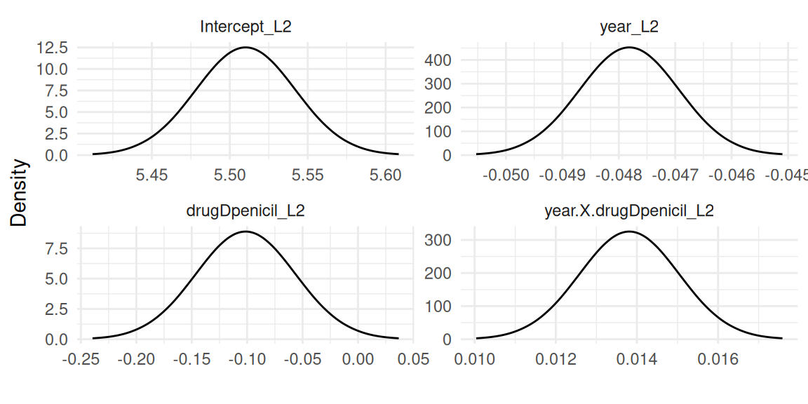
Intercept_L2 5.5102 0.0319 5.4476 5.5102 5.5727
year_L2 -0.0478 0.0009 -0.0495 -0.0478 -0.0461
drugDpenicil_L2 -0.1014 0.0449 -0.1893 -0.1014 -0.0134
year:drugDpenicil_L2 0.0138 0.0012 0.0114 0.0138 0.0162
Random effects variance-covariance
mean sd 0.025quant 0.5quant 0.975quant
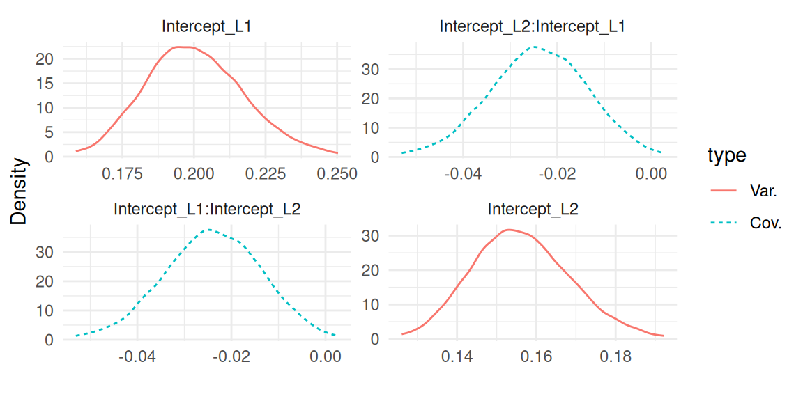
Intercept_L1 0.2004 0.0176 0.1689 0.1993 0.2374
Intercept_L2 0.1560 0.0128 0.1325 0.1551 0.1837
Intercept_L1:Intercept_L2 -0.0236 0.0109 -0.0459 -0.0231 -0.0035
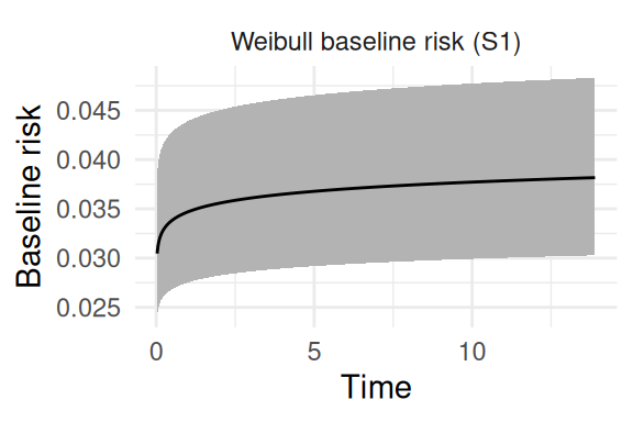
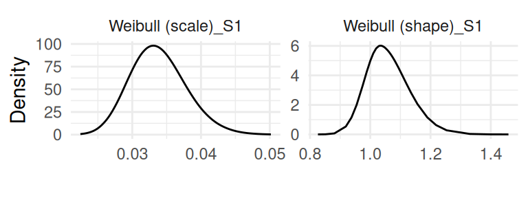
Survival outcome
mean sd 0.025quant 0.5quant 0.975quant
Weibull (shape)_S1 1.0603 0.0716 0.9376 1.0544 1.2183
Weibull (scale)_S1 0.0338 0.0041 0.0265 0.0336 0.0425
drugDpenicil_S1 0.1139 0.1716 -0.2224 0.1139 0.4502
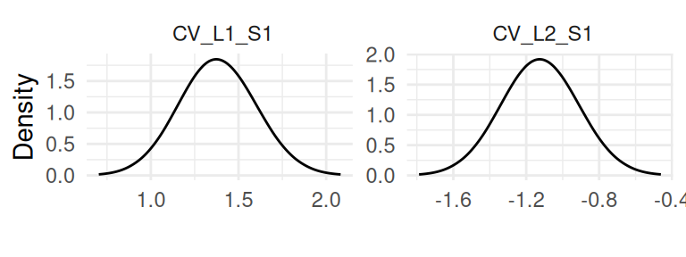
Association longitudinal - survival
mean sd 0.025quant 0.5quant 0.975quant
CV_L1_S1 1.3816 0.2237 0.9458 1.3800 1.8267
CV_L2_S1 -1.1248 0.2152 -1.5476 -1.1251 -0.7003
log marginal-likelihood (integration) log marginal-likelihood (Gaussian)
-45028.67 -45021.94
Deviance Information Criterion: 45454.22
Widely applicable Bayesian information criterion: 81938.44
Computation time: 7.47 secondsThe results printed starts with parameters related to the first longitudinal outcome (SGOT), including fixed effects and the standard deviation of the residual error. Then the parameters corresponding to the second longitudinal outcome (platelets) are displayed and below is the variance-covariance of random effects. Parameters related to the survival outcome are then displayed, with the shape and scale of the Weibull distribution for the baseline hazard and the fixed effect of trt (i.e., drug).
Finally, the association parameters for the current value of the two shared linear predictors to scale their effect on the risk of event are displayed. The names of outcomes are conveniently named with the letter “L” for longitudinal outcomes and “S” for survival outcomes followed by their position in the list of formulas, allowing to easily identify the involved components for association parameters and when plotting and doing predictions. The marginal likelihood of the model and some goodness of fit criteria are provided at the end of the summary function (i.e., DIC, WAIC).
As illustrated in the next call, adding the argument sdcor=TRUE to the call of the summary function returns standard deviations of the residual error and the random effects as well as correlation between random effects instead of the default variance and covariance as illustrated in the previous call. Moreover, parameters related to the risk of event can be transformed to hazard ratios by adding the argument hr=TRUE (default is FALSE) to the call of the summary function, which properly propagates uncertainty from the log scale. We can print the summary with these two options:
summary(IJ, sdcor=TRUE, hr=TRUE)Longitudinal outcome (L1, lognormal)
mean sd 0.025quant 0.5quant 0.975quant
Intercept_L1 4.7972 0.0388 4.7212 4.7972 4.8733
year_L1 -0.0051 0.0038 -0.0126 -0.0051 0.0024
drugDpenicil_L1 -0.1546 0.0546 -0.2616 -0.1546 -0.0475
year:drugDpenicil_L1 -0.0014 0.0053 -0.0118 -0.0014 0.0091
Res. err. (sd) 0.3070 0.0053 0.2967 0.3070 0.3176
Longitudinal outcome (L2, poisson)
mean sd 0.025quant 0.5quant 0.975quant
Intercept_L2 5.5102 0.0319 5.4476 5.5102 5.5727
year_L2 -0.0478 0.0009 -0.0495 -0.0478 -0.0461
drugDpenicil_L2 -0.1014 0.0449 -0.1893 -0.1014 -0.0134
year:drugDpenicil_L2 0.0138 0.0012 0.0114 0.0138 0.0162
Random effects standard deviation / correlation
mean sd 0.025quant 0.5quant 0.975quant
Intercept_L1 0.4473 0.0197 0.4098 0.4468 0.4867
Intercept_L2 0.3948 0.0158 0.3648 0.3941 0.4262
Intercept_L1:Intercept_L2 -0.1364 0.0580 -0.2491 -0.1362 -0.0250
Survival outcome
exp(mean) sd 0.025quant 0.5quant 0.975quant
Weibull (shape)_S1 1.0603 0.0716 0.9376 1.0544 1.2183
Weibull (scale)_S1 0.0338 0.0041 0.0265 0.0336 0.0425
drugDpenicil_S1 1.1367 0.1931 0.8037 1.1204 1.5616
Association longitudinal - survival
exp(mean) sd 0.025quant 0.5quant 0.975quant
CV_L1_S1 4.0789 0.9113 2.5917 3.9718 6.1642
CV_L2_S1 0.3321 0.0710 0.2141 0.3245 0.4927
log marginal-likelihood (integration) log marginal-likelihood (Gaussian)
-45028.67 -45021.94
Deviance Information Criterion: 45454.22
Widely applicable Bayesian information criterion: 81938.44
Computation time: 7.47 secondsNow we can have a more interpretable output, for example the variability of the range of values for the second random intercept is approximately twice its standard deviation, meaning that we expect ~95% of the values between around -0.8 and 0.8. For the hazard ratio, we can see that a one unit increase in the second marker’s linear predictor value is associated to a risk of event multiplied by 4 [95% credible interval: 2.59 - 6.17].
1.5.4 Plot function
The plot function, when applied to an object fitted with INLAjoint returns the marginal posterior distributions of all the model parameters as well as baseline hazard parameters and baseline hazard curves for survival models. The R package ggplot2 (Wickham (2016)) is used within INLAjoint for these plots:
plot(IJ)The first plots returned contains the fixed effects and likelihood family parameters for each outcome, starting with the first outcome which is here a lognormal mixed-effects model (Figure 1.1):
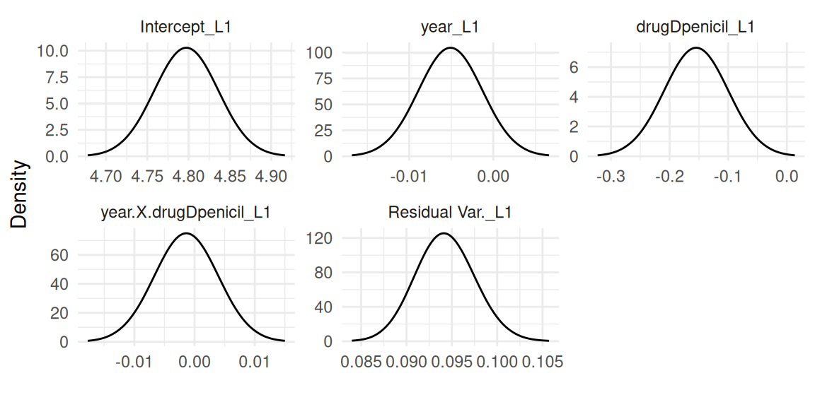
Then the second outcome which is the Poisson mixed-effects model (Figure 1.2):
Finally the survival outcome modeled with proportional hazards (Figure 1.3):
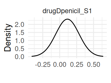
Figure 1.4 shows the variance and covariance of the random effects:
All the association parameters are grouped in Figure 1.5:
And the remaining plots are for the baseline, starting with the baseline hazard curve (Figure 1.6):
and the baseline parameters (Figure 1.7):
It is also possible to switch from variance and covariance of residual error terms and random effects to standard deviations and correlations with the argument sdcor. The boolean priors allows to add the prior distribution on each posterior distribution plot, which is very useful to identify parameters that may rely mostly on the prior (i.e., the observed data is not informative) and to do prior sensitivity analysis to assess the impact of priors on the posteriors.
It is not always easy to understand the implication of priors in Bayesian inference and this tool allows for visualisation of their distribution and impact on the results. Evaluating the impact of priors on the results of a Bayesian model by looking at the posterior obtained from different priors can avoid wrong conclusion due to misleading priors and this tool facilitates this process. We can illustrate these two features with Figure 1.8:
plot(IJ, sdcor=TRUE, priors=TRUE)$Covariances$L1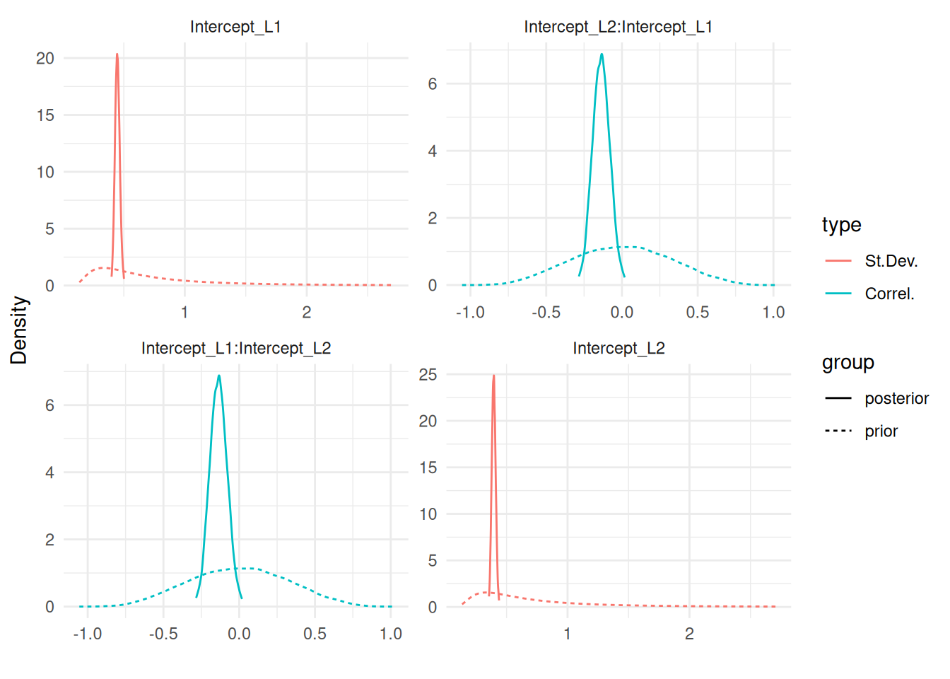
1.5.5 Predict function
The predict function is an important component of INLAjoint. It is designed for three primary tasks:
- Inference, such as visualizing average treatment effects across different scenarios.
- Dynamic predictions, to predict patient-specific outcomes and update as new information becomes available.
- Imputation, to obtain estimates of missing values.
Whether the user has fitted a longitudinal-only model, a survival-only model or a joint model with multiple outcomes, the same function is used to generate predictions. The predict function reframes the fitted model from a static summary of parameters into a dynamic tool.
It uses a simple syntax that requires a fitted model and new data to compute the model predictions for all the outcomes included in a model, based on the new data.
The computations of predictions for a new subject, say subject \(i\), who was not part of the original dataset \(D_n\) used to fit the model, presents a specific statistical challenge. For individualized predictions, we need to estimate the subject-specific random effects, denoted \(b_i\), conditioned on their unique and often sparse longitudinal history, \(Y_i(t)\). This requires integrating over the uncertainty of both the population-level parameters (which include fixed effects, variance-covariance parameters, etc.) and the individual-specific random effects.
The predict function in INLAjoint first draws a sample of the population-level parameters from their approximated posterior distributions. For each sampled set of population parameters the function uses the INLA method to treat the new subject’s data as an inference problem where the objective is to get the individual’s random effect posterior based on the new data for each set of sampled population parameters.
The horizon argument allows to choose the horizon of the prediction, it can be set as a vector with different values for different prediction tasks. With default options, the predict function returns the value of the linear predictor for each id in the new data provided at a number of time points that can be defined with argument NtimePoints (default 50 equidistant time points between 0 and maximum time). It is however possible to choose the time points manually with the argument timePoints.
Uncertainty is quantified through sampling, where the number of samples for hyperparameters and fixed effects is defined by the argument NsampleHY (default 20) and NsampleFE (default 20), respectively. Note that each hyperparameter sample includes NsampleFE samples of fixed effects, so default is \(20*20=400\) samples for fixed effects. For each sample, random effects realizations are sampled conditional on the observed data in the new dataset provided. The number of random effects nested samples can be chosen with the argument NsampleRE (default 50). Here also, each sample of fixed effects is associated to NsampleRE samples of random effects, so the default number of random effects samples is \(400*50=20000\).
The default values have been defined based on simulations, aiming at providing an optimal tradeoff between accuracy of the predictions and computation time. Since we sample random effects conditional on the observed data, the number of required samples to properly measure uncertainty is reduced compared to other approaches that samples from the marginal distribution of random effects and weight each sample with the probability density of the sample compared to the new observed data.
Indeed, internally the predict function uses the INLA algorithm to compute the posterior distribution of the random effects conditional on the new data, from which we can sample to capture the individual-level uncertainty source.
The default output of the predict function returns summary statistics over the linear predictor of each outcome but it is possible to get the sampled curves instead by switching the boolean argument return.samples to TRUE (see Section 2.9).
We can create a simple one-line dataset to define the scenario we want to predict for:
  id      drug year SGOT platelets
1  1 D-penicil    0   NA        NA
The dataset gives a unique id for the prediction scenario id. It is useful when we want to include multiple lines of data for one scenario as illustrated later in this section but it is important to note here that this id is not the same as the id used in the model fit, i.e., id=1 here does not mean this is the same individual as id 1 in the original dataset, the predict function always assume individuals are new individuals.
Predictions for an id that we already learned from during the estimation process is handled differently (see Section 5.1 for an example of a prediction for an individual that is characterized by an already existing random effect group). If the prediction task involves an individual from the learning set that has some new observed data, one can include all the data history in the newData argument of the predict function and thus treat him as a new individual. An alternative consists in including this individual’s time points at which we want to predict in the learning set, with outcome set to NA, since INLA will compute the expected value of the outcome during the inference process automatically.
In addition to the id, the new data we created for the prediction also includes a value for each covariate in the model, here we have trt and year (which is only used when some outcome measures are included to know the measurement time) and a value for each longitudinal outcome which here are both set to NA, meaning that we want the marginal prediction for trt=1 (i.e., not conditional on anything else than trt).
P <- predict(IJ, newData = NewData, horizon = 14, id = "id")The first argument is the model from which we derive predictions (IJ), the second argument is the new dataset that gives the scenarios of interest (i.e., here we want to compute the hazard function for trt=1). The argument horizon gives the time until which we want to compute the predictions and the argument id gives the column name for scenarios.
str(P)List of 2
$ PredL:'data.frame': 100 obs. of 8 variables:
..$ id : Factor w/ 1 level "1": 1 1 1 1 1 1 1 1 1 1 ...
..$ year : num [1:100] 0 0.286 0.571 0.857 1.143 ...
..$ Outcome : chr [1:100] "SGOT" "SGOT" "SGOT" "SGOT" ...
..$ Mean : num [1:100] 4.63 4.63 4.62 4.62 4.62 ...
..$ Sd : num [1:100] 0.451 0.451 0.451 0.451 0.451 ...
..$ quant0.025: num [1:100] 3.75 3.75 3.74 3.74 3.74 ...
..$ quant0.5 : num [1:100] 4.63 4.62 4.62 4.62 4.62 ...
..$ quant0.975: num [1:100] 5.51 5.51 5.51 5.51 5.5 ...
$ PredS:'data.frame': 50 obs. of 8 variables:
..$ id : Factor w/ 1 level "1": 1 1 1 1 1 1 1 1 1 1 ...
..$ year : num [1:50] 0 0.286 0.571 0.857 1.143 ...
..$ Outcome : chr [1:50] "S_1" "S_1" "S_1" "S_1" ...
..$ Haz_Mean : num [1:50] 0.214 0.215 0.216 0.218 0.219 ...
..$ Haz_Sd : num [1:50] 0.456 0.458 0.461 0.463 0.466 ...
..$ Haz_quant0.025: num [1:50] 0.000675 0.000684 0.000692 0.000701 0.000709 ...
..$ Haz_quant0.5 : num [1:50] 0.0481 0.0486 0.049 0.0494 0.0498 ...
..$ Haz_quant0.975: num [1:50] 1.43 1.44 1.46 1.46 1.47 ...The result is a list of two data frames, where the first one predL includes the prediction for the longitudinal outcomes with columns id to identify the scenario, year for the measurement time, Outcome for the outcome (the data frame includes first the predictions of the first longitudinal outcome at 50 time points followed by the second longitudinal outcome at the same time points), and then summary statistics over the linear predictors. Similarly, in the second element of the list, PredS, we have the predictions of the survival outcome at the same 50 time points.
We can plot the predicted longitudinal and survival trajectories (Figure 1.9 and Figure 1.10):
library(ggplot2)
ggplot(P$PredL, aes(x = year, y = quant0.5)) + facet_wrap(~Outcome+id) +
  geom_line() + xlab("Time") + ylab("Linear predictor") +
  geom_line(aes(y = quant0.025),linetype="dotted") +
  geom_line(aes(y = quant0.975),linetype="dotted") +
  theme(legend.position="bottom") + theme_minimal()
ggplot(P$PredS, aes(x = year, y = Haz_quant0.5)) +
  geom_line() + xlab("Time") + ylab("Event hazard") +
  geom_line(aes(y = Haz_quant0.025),linetype="dotted") +
  geom_line(aes(y = Haz_quant0.975),linetype="dotted") +
  theme(legend.position="bottom") + theme_minimal()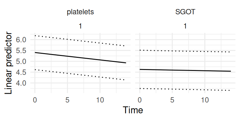

These trajectories represent the linear predictor for each outcome, they can however be transformed to get a more interpretable scale as illustrated later in this section. The risk function here shows quite large uncertainty which is due to the small sample size used for this illustration. Many other prediction examples are provided in the rest of the book, showing how uncertainty depends on the model complexity as well as the data information.
The boolean argument survival allows to compute summary statistics over survival curves in addition to the risk curves. Note that in order for the survival probabilities to be accurate, since the survival function is based on the cumulative hazard function (i.e., integrated hazard function), many time points must be included during the at-risk period, since these time points are used to approximate numerically the cumulative hazard function.
Therefore if we are only interested in the survival probability at horizon time, it is important to have many time points between the entry in the at-risk period and the horizon time to get accurate predictions. For joint models with default options, survival predictions assume the individual did not experience the survival event(s) before the last longitudinal observation provided in the new dataset (time 0 if the predictions are only conditional on baseline covariates, as in the previous example).
However, it is possible to manually define the time point at which survival prediction should start with the argument Csurv (i.e., we fix the entry in the at-risk period), as illustrated later in this section and in Section 2.2.3. When fitting a competing risks model, the boolean argument CIF allows to compute the cumulative incidence function instead of survival, which is more interesting to interpret as survival curves represents the probability of having an event in a hypothetical world where it is not possible to have any of the competing events while the cumulative incidence functions give the probability of observing an event accounting for the fact that subjects may have one of the competing events before (see Section 2.8).
For a longitudinal outcome, the argument inv.link allows to apply the inverse link function in order to get predictions on a more interpretable scale and to allow for observed vs. fitted of non-Gaussian outcomes. For example for a binomial model for binary data with a logit link, when inv.link is set to TRUE in the call of predict, the returned predictions give the probability of 1 versus 0 instead of the predicted linear predictor, with uncertainty quantification on this scale. This feature allows to directly interpret and display the results on the scale of the observed data (see Section 3.3.1 and Section 3.3.2).
While it is possible to use the predict function to predict the longitudinal and survival models trajectories over new individuals or forecast for some known individuals, it also allows to predict the average trajectory for any outcome conditional on covariates as we just illustrated. In this case, the new data should only consist of one line that gives the value of covariates and the longitudinal outcomes values should be set to NA or not given at all. The predict function will automatically assume the average trajectory of each outcome conditional on the given covariates, and will quantify uncertainty through sampling from marginal distributions which allows to display the average trajectories for inference purposes.
This is very useful for complex models as it is common to use models that allow for complex trajectories (e.g., fixed and random effects on splines or complex interactions), where the value of parameters is difficult to directly interpret. With this feature, one can compute the average trajectory conditional on a covariate such as treatment and compare the longitudinal and survival profiles of each treatment line visually for example.
We can compute predictions for the same scenario as the previous example with the same model but adding some of the arguments we just introduced. Let’s consider the first 6 individuals in the fitted dataset (treated as new individuals for simplicity). Here we print the first couple lines of the new dataset:
  id      drug      year  SGOT platelets
1  1 D-penicil 0.0000000 138.0       190
2  1 D-penicil 0.5256817   6.2       183
3  2 D-penicil 0.0000000 113.5       221
4  2 D-penicil 0.4983025 139.5       188
5  2 D-penicil 0.9993429 144.2       161
6  2 D-penicil 2.1027270 144.2       122
These individuals have longitudinal measurement of both our outcomes of interest recorded. We may want to predict the expected value of each longitudinal outcome conditional on these measurements as well as corresponding survival probabilities. We set the horizon to be different for each individual (we predict at horizon 9 for first individual, 10 for second individual, etc.). We also assume the survival probabilities are computed conditional on the fact that the entry in the at-risk period is at time 1 for all individuals (argument Csurv):
P <- predict(IJ, NewData, horizon = 9:14, id="id",
             survival=TRUE, inv.link=TRUE, Csurv=1)
We can plot the predicted longitudinal trajectories for each individual, for example for the first outcome (platelets), and we can add the observed repeated measurements that have been taken into account to make individualized predictions (Figure 1.11):
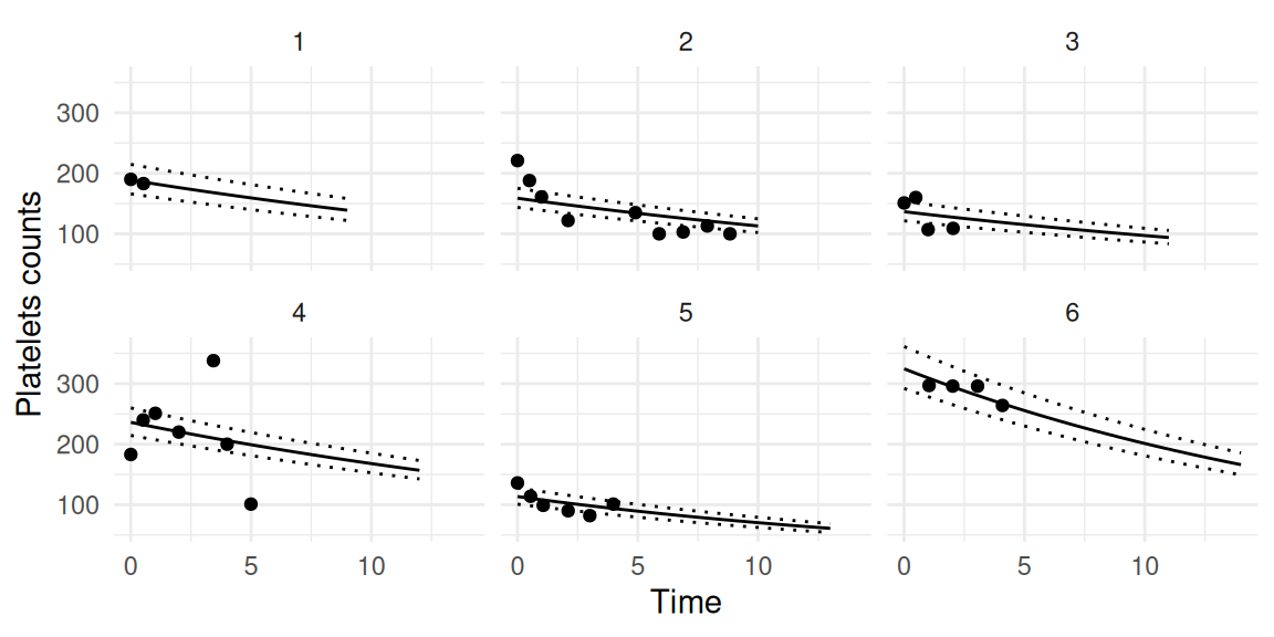
As we can see, for each individual we get the estimated counts based on the Poisson rate after applying the inverse link function. We can also display the corresponding survival probabilities (Figure 1.12):
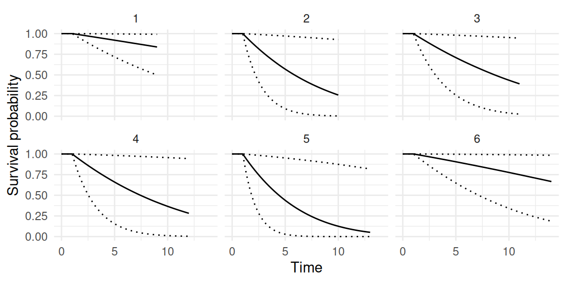
Here, despite the large uncertainty, we can see that all individuals enter the at-risk period after 1 unit of time and the horizon of the prediction is individual-specific (it can be common to all individuals if an unique value is provided instead of a vector).
Note that predictions with INLAjoint are fully Bayesian, meaning that all the parameters are sampled to assess uncertainty while many methods use empirical Bayes predictions (where hyperparameters are not sampled). However, the predict function can be configured to compute empirical Bayes predictions by setting the argument NsampleHY to 1 (then the number of fixed effects NsampleFE should be increased to 400 to keep consistent accuracy).
Summary metrics of predictive accuracy, such as the time-dependent Receiver Operating Characteristic Area Under the Curve (ROC AUC) or the Brier score, are not directly implemented in INLAjoint. This is a deliberate design choice, as statistically rigorous implementations (that properly account for censoring) are already available in dedicated external tools, which can efficiently process predictions generated by INLAjoint. A state-of-the-art example of this approach is the methodology proposed by Blanche et al. (2015), which uses Inverse Probability of Censoring Weight (IPCW) to compute unbiased estimates of dynamic AUC and Brier scores.
1.5.6 Sampling from the posterior distributions
It is possible to sample marginalized fixed effects realizations of any model (i.e., hyperparameters integrated out) with the function inla.rjmarginal(N, MODEL), where N is the number of samples and MODEL is a fitted model with INLAjoint. To sample hyperparameters, the function inla.hyperpar.sample(N, MODEL) can be used similarly.
1.5.7 Highest posterior density intervals
While the default credible intervals in R-INLA and INLAjoint are based on quantiles, highest density intervals are easily computed from the posterior marginals using the inla.hpdmarginal() function from the R-INLA package. We can compare the default quantile-based credible interval to highest density interval on the shape parameter of the Weibull distribution used for the baseline hazard of the example in Section 1.5.2. We select this parameter due to its skewed posterior, to better illustrate the differences since the intervals are identical on symmetric distributions.
hpd_interval <- inla.hpdmarginal(0.95, IJ$marginals.hyperpar[[2]])
par(mar = c(3,0.5,3,0.5), cex.lab=0.1)
plot(IJ$marginals.hyperpar[[2]], type = 'l',
     ylab = "Density", xlab = "Weibull Shape Parameter",
     main = "95% highest density vs. quantile-based
     interval for a skewed posterior", yaxt = "n")
abline(v = hpd_interval, col = 2, lty = 2, lwd=3)
abline(v = IJ$summary.hyperpar[2,c(3,5)], col = 4, lty = 3, lwd=3)
legend("topright", legend = c("highest density", "quantile-based"),
       col = c(2,4), lty = 2:3, lwd=3)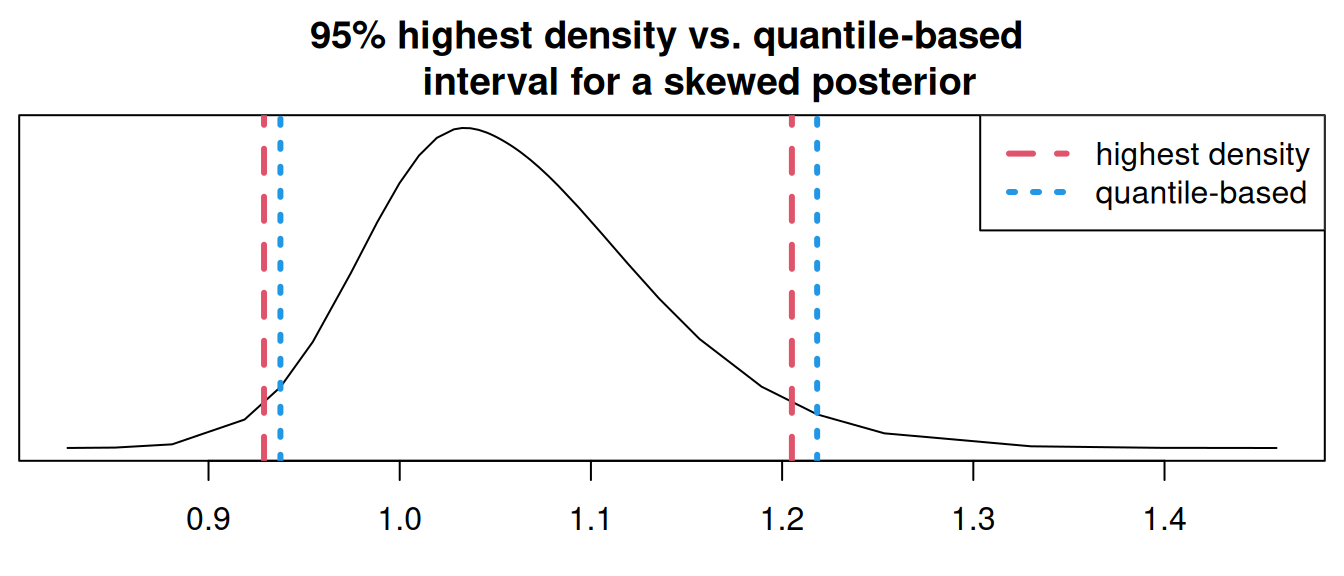
1.5.8 Build only option
It is possible to build the structure of a model with INLAjoint by setting the argument run=FALSE in the call of the joint() function, which creates an object with all the components required to run the INLA algorithm but does not run the algorithm. This allows to make modifications to the model before running it, which can be useful to make some R-INLA specific modifications that cannot be made directly with INLAjoint. Multiple examples of the use of this option are given in the rest of the book (See Section 2.12.1, Section 3.5, Section 3.7, Section 3.9, Section 4.3.6 and throughout Chapter 5). Thanks to this feature, one can take advantage of the user-friendliness of INLAjoint to build a complex multivariate model and also benefit from all the flexibility of R-INLA to tailor the model to the user’s needs without being limited by the current state of the implementations in INLAjoint.
1.6 Performance evaluation of INLA
The INLA methodology calculates approximations to the marginal posteriors and as such an approximation error will inherently exist. Since the inception of the INLA methodology it has been compared with MCMC methods, considered as the gold standard, and shown to exhibit exceptional accuracy. In the case of survival, longitudinal and joint models, it has been shown by Martino et al. (2011), Van Niekerk, Bakka, et al. (2023), Van Niekerk et al. (2021), Rustand et al. (2023), Alvares et al. (2024), that the approximated posterior density functions closely match those obtained from long MCMC runs. The frequentist properties such as the bias and coverage of the posterior estimates for joint models, calculated with the INLA methodology, was investigated by Rustand, Van Niekerk, et al. (2024), and the procedure was shown to possess good frequentist properties in terms of the bias while attaining the desired level of nominal coverage of the credible intervals.
As an illustration of the relative performances of INLA compared to MCMC, we can fit the model from Section 1.5.2 with MCMC and compare results and computation time. Details about this comparison are provided in Rustand, Niekerk, et al. (2024), here we only focus on the results to illustrate the significant potential of INLA for the joint analysis of longitudinal and survival data.
We consider two available MCMC alternatives in R able to fit this model: JMbayes2 (version 0.5-7) and rstanarm (version 2.32.1). Note that JMbayes2 and rstanarm use maximum likelihood estimates from univariate models (i.e., mixed-effects and proportional hazards models) to define initial values and JMbayes2 also uses those univariate models to define data-driven prior distributions for the joint model fit, thus giving an intrinsic advantage to the MCMC methods over the INLA approach that use non-informative initial values and priors.
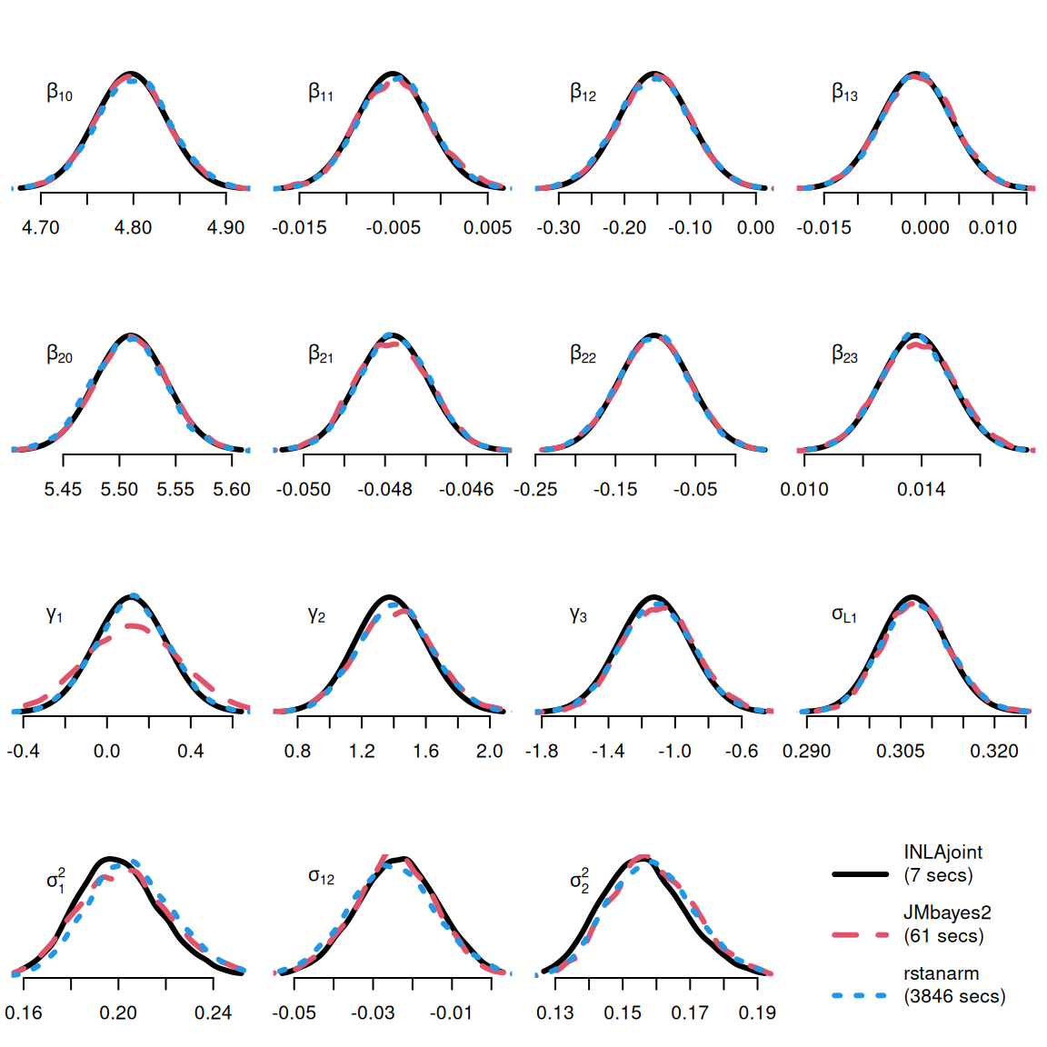
Figure 1.13 shows that INLAjoint gives similar results as the MCMC-based packages, but with exceptional computational efficiency. This illustrates how INLAjoint facilitates the application of joint models, as their use has been restrained by their computational burden coming from both the random effects and the time-dependent association structures. INLA allows for more complex models and large data applications at a reasonable computational cost.