library(rnaturalearth) # map data
fr0<-ne_states("france")
fr1 <- fr0[fr0$type!="Overseas département" & fr0$region!="Corse",]
dim(fr1)
[1] 94 122In the previous chapters, we assumed the independence of observations, conditional on the model’s fixed and random effects. The random effects considered were restricted to be independent across individuals but correlated within an individual. However, in some biomedical and epidemiological studies, group level heterogeneity might be present. For instance, health outcomes sometimes exhibit geographical patterns. Factors such as environmental exposures, socioeconomic disparities, cultural behaviors or different access to healthcare can create spatial structures where individuals in nearby areas are more similar to each other than to individuals in distant areas. This is known as spatial autocorrelation.
Spatial autocorrelation violates the independence assumption of standard regression models. The model may incorrectly attribute spatially structured variation to a measured covariate, leading to biased estimates and wrong conclusions. To address this, we introduce spatial random effects, which are latent variables designed to explicitly model and account for unmeasured, spatially varying risk factors.
Spatial random effects rely on sharing information between nearby geographical units (i.e., spatial smoothing). For example an area with a small population or sparse data may produce unstable, high-variance estimates of an event risk. A spatially structured random effect can use information from neighboring areas to improve the stability of the estimate for the location of interest.
INLA has been widely developed in the field of spatial statistics and there are many options available. In this chapter, we only introduce the main spatial random effects that could be used in practice as random effects in survival, longitudinal or joint models. The first two sections focus on areal data, where observations are aggregated over discrete geographical regions, such as municipalities or regions. For this type of data, we will introduce models based on neighborhood structures, including the Besag and the Besag-York-Mollié (BYM) models. The final section focuses on point referenced data where each observation is associated with a specific set of coordinates, such as a patient’s home address or the location of a pollution sensor. For this continuous spatial setting, we will use the Stochastic Partial Differential Equation (SPDE) approach.
These spatial random effects are not directly implemented in INLAjoint, but we use INLAjoint to define the model structure and construct relevant design matrices whereafter we include the spatial random effect, and fit the model using R-INLA (see Section 1.5.8). This is one instance of how we can combine the flexibility of the INLA methodology, and all available specific options tailored for R-INLA, with the user-friendly INLAjoint framework.
In disease mapping and spatial epidemiology it is common to encounter data that is aggregated by geographical areas, such as municipalities. In this setting, we can account for the spatial correlation by a spatially structured random effect at the areal unit level. Therefore, all the individuals within an area share the same random effect. Common models used in this setting are based on the conditional autoregressive (CAR) model (Besag (1974)). The CAR model considers conditional distributions based on neighboring regions, where the random effect in a given area is modeled as a weighted average of the random effects in its neighboring areas, which gives a spatially structured random effect where neighboring regions are more similar than distant ones.
The original parametrization for the CAR model given in Besag (1974) for regular lattices, has been adapted and used in the context of irregular geographic areal maps such as cities. We consider the spatial effect for area \(s\), \(b_s\), for \(s\in \{1, \ldots, m\}\) considering a total of \(m\) areas in the map. In this setting, the conditional distribution of \(b_s\) (i.e., conditional on the neighboring areas) is \[ b_s|\sigma_c^2 \sim \textrm{N}(\overline{b}_s, \sigma_c^2/n_s) \] where \(\overline{b}_s=\rho\sum_{k\sim s}b_k\) with \(k\sim s\) meaning that area \(k\) is neighbor to area \(s\), \(n_s\) is the number of neighbors of area \(s\), \(\rho\) is an autocorrelation parameter, and \(\sigma_c^2\) is the conditional variance parameter.
This model belong to the Gaussian Markov Random Field (GMRF) class of models (Rue & Held (2005)), where the specification of the joint distribution is derived from the set of conditional distributions. The distribution of the entire vector or spatial random effects \(b_s=\{b_1, ...,b_m\}\) is a multivariate Gaussian distribution with zero mean vector and a precision matrix given by \[ Q = \frac{1}{\sigma_c^2}(D-\rho \cdot G) \] The matrix \(D\) is a diagonal matrix where \(D_{ss}=n_s\) and \(G\) is a matrix where \(G_{sk}=1\) if \(k\sim s\) or \(0\) (zero) otherwise. While several variations of the CAR model exist, we will focus on its most common formulation that is implemented in INLA.
The intrinsic conditional autocorrelation (ICAR) model is a particular case of the CAR model when \(\rho=1\). This assumption means that the model is defined by the differences between the effects of neighboring areas. The joint distribution is then said to be improper (i.e., it does not integrate to one) and its precision matrix is rank-deficient. To ensure the model is identifiable, a sum-to-zero constraint is defined (\(\sum_{s=1}^{m} b_s = 0\)) which fixes the overall mean of the spatial effects at zero.
Therefore, under ICAR we have \[ b|\sigma_c^2, R \sim \textrm{N}(0, \sigma_c^2 \cdot R^{-}) \] where \(R^{-}\) is the generalized inverse of \(R\), which is defined from the neighborhood structure as \(R_{ss} = n_s\), and \(R_{sk}\), for \(k\neq s\), is \(-1\) if \(k \sim s\) or \(0\) otherwise. As often done within the INLA framework, we will refer to the ICAR model as the Besag model from now on.
The interpretation of the conditional variance parameter \(\sigma_c^2\) is not very useful as it depends on the neighborhood structure of the map. We shall scale the matrix \(R\) as proposed in Sørbye & Rue (2014), so that we can interpret the variance parameter. Let the scaled matrix be \(R^{*}=g_R \cdot R\), where \(g_R\) is the geometric mean of the non-zero eigenvalues of \(R\). Therefore \(R^{*}\) is so that the geometric mean of the diagonal elements of its (generalized) inverse is equal to one. In this case we consider the joint distribution of \(b\) as \[\begin{equation} b|\sigma^2, R^* \sim \textrm{N}(0, \sigma^2 \cdot (R^{*})^{-}) \end{equation}\] where \(\sigma^2\) is a marginal variance parameter, which is easier to interpret than \(\sigma_c^2\).
In order to illustrate the Besag model, let’s first consider a map. We can use a map of mainland France available in the R package rnaturalearth (Massicotte & South (2023)):
library(rnaturalearth) # map data
fr0<-ne_states("france")
fr1 <- fr0[fr0$type!="Overseas département" & fr0$region!="Corse",]
dim(fr1)[1] 94 122The map is decomposed into 94 departments, we can plot the map with the R package ggplot2 (Wickham (2016)):
library(ggplot2) # to plot
ggplot() + geom_sf(data = fr1) + theme_minimal()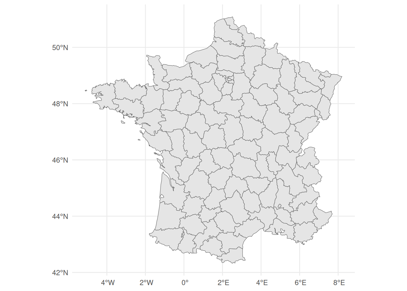
We can use the R package spdep (Bivand et al. (2013)) to build the neighbor list, which gives for each department the corresponding neighbors:
library(spdep)
nblist <- poly2nb(fr1);nblist
Neighbour list object:
Number of regions: 94
Number of nonzero links: 478
Percentage nonzero weights: 5.409688
Average number of links: 5.085106 We can convert the map to the INLA format, where the matrix Graph gives the neighbor structure, i.e., each line is a department and the squares in the column indicates corresponding neighbors (Figure 5.2):
library(INLA)
graph.file <- "graph.file"
nn <- card(nblist)
n.areas <- length(nn)
nb2INLA(file = graph.file, nb = nblist)
inlaGraph <- inla.read.graph(graph.file)
Graph <- sparseMatrix(i=rep(1:length(nn),nn), j=unlist(nblist[nn>0]), x=1)
par(mar = c(0, 0, 0, 0))
image(matrix(Graph, ncol = 94), axes = F, asp = 1)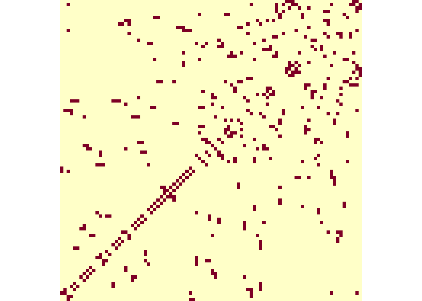
We can then simulate a spatial random effect for each department, where we assume some spatial structure (i.e., correlation between neighbors). The function inla.qsample allows to simulate from the spatial random effect given its precision matrix. We consider a precision of 1 (i.e., standard deviation also equals 1) for this spatial random effect:
tau.spatial <- 1 # spatial random effect precision
R <- Diagonal(n = length(nn), x = nn) - Graph
sconstr <- list(A = matrix(1, 1, nrow(R)), e = 0)
R.scaled <- inla.scale.model(Q = R+Diagonal(nrow(R))*1e-5, constr=sconstr)
s.besag <- inla.qsample(n = 1, Q = R.scaled*tau.spatial,
                         constr=sconstr, seed=4)
ggplot() + geom_sf(data = fr1, aes(fill = s.besag))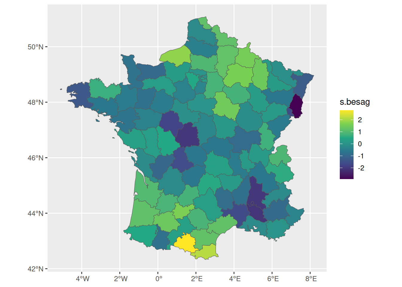
We can define a survival model where each individual belong to a department with an associated risk, then we can include a spatially structured random effect to capture this risk on the department level in addition to the effect of some measured covariates such as treatment: \[\lambda_{i}(t)=\lambda_{0}(t)\ \textrm{exp}\left(\gamma\cdot trt_i + b_{s(i)}\right)\] where \(b_{s(i)}\) is a random effect at the (areal) department level for individual \(i\) such that \(s(i)\in\{1,2,...,m\}\). This random effect has been simulated (s.besag) and displayed in Figure 5.3. We can use it to simulate some data from this model, let’s consider 2000 individuals randomly assigned to one of the departments:
n=2000 # number of individuals
gamma_1=0.2 # treatment effect
baseScale=0.5 # baseline hazard scale (Weibull distribution)
baseShape=1.3 # baseline hazard shape (Weibull distribution)
followup=4 # study duration
trt <- rbinom(n, 1, 0.5) # treatment covariate
id_s <- sample(1:n.areas, n, replace = TRUE) # assign departments
u <- runif(n) # uniform distribution for survival times generation
eventTimes <- (-(log(u))/(baseScale*exp(trt*gamma_1 +
                                        s.besag[id_s])))^(1/baseShape)
eventIndic <- as.numeric(eventTimes<followup)
eventTimes <- pmin(eventTimes, followup)
datSbesag <- data.frame(id=1:n, eventTimes, eventIndic, trt, id_s)
str(datSbesag) # data
'data.frame': 2000 obs. of 5 variables:
$ id : int 1 2 3 4 5 6 7 8 9 10 ...
$ eventTimes: num 1.2093 0.2418 0.1381 0.8444 0.0349 ...
$ eventIndic: num 1 1 1 1 1 1 1 0 1 1 ...
$ trt : int 0 1 1 0 1 1 0 1 0 1 ...
$ id_s : int 64 4 23 29 86 24 4 20 82 76 ...We now have time-to-event data at the individual level (id), where each individual is associated to one of the departments (id_s). Now we can use INLAjoint to build the necessary design matrices. We include an iid random effect in the survival model as illustrated in Section 2.10, while enabling the “build only” feature introduced in Section 1.5.8, such that we can setup the design matrix for the random effect to make it a spatially structured Besag before running INLA:
library(INLAjoint)
M_bs0 <- joint(formSurv = list(inla.surv(eventTimes,
                                         eventIndic) ~ trt + (1|id_s)),
               dataSurv = datSbesag, id = "id_s", run = FALSE)
M_bs0$.args$formula <- as.formula(paste(c("Yjoint ~ -1 ",
      attr(terms(M_bs0$.args$formula), which = "term.labels")[1:3],
      "f(IDIntercept_S1, model='besag', graph=Graph, scale.model=TRUE)"),
                                         collapse = "+"))
Here the model has been setup in M_bs0 but INLA was not run because we included the argument run = FALSE. We can modify the formula to remove the iid random effect and replace it with the Besag random effect before running INLA. This conveniently allows to reuse the same id IDIntercept_S1 as initially setup for the iid effect, then the model is defined as besag, the graph for the spatial structure is Graph and we scale the model such that the random effects sums to zero. We can run the model with the joint.run() function:
M_bs <- joint.run(M_bs0)
summary(M_bs)
Survival outcome
                           mean     sd 0.025quant 0.5quant 0.975quant
Baseline risk (variance) 0.0539 0.0280     0.0184   0.0476     0.1265
trt                      0.2122 0.0494     0.1153   0.2122     0.3091

Frailty term variance
             mean     sd 0.025quant 0.5quant 0.975quant
IDIntercept 0.916 0.1563     0.6494   0.9023     1.2625

log marginal-likelihood (integration)    log marginal-likelihood (Gaussian)
                            -6462.674                             -6462.234

Deviance Information Criterion:  12673.67
Widely applicable Bayesian information criterion:  12673.72
Computation time: 1.42 seconds
The frailty term variance here corresponds to the variance of our Besag random effect. Figure 5.4 shows the posterior distribution of treatment effect and the baseline hazard (simulated as Weibull but estimated with a random walk):
library(ggpubr) # for ggarrange layout
trt_S1 <- plot(M_bs)$Outcomes$S1
trt_S1$data <- trt_S1$data[trt_S1$data$Effect=="trt_S1",]
ggarrange(trt_S1, plot(M_bs)$Baseline)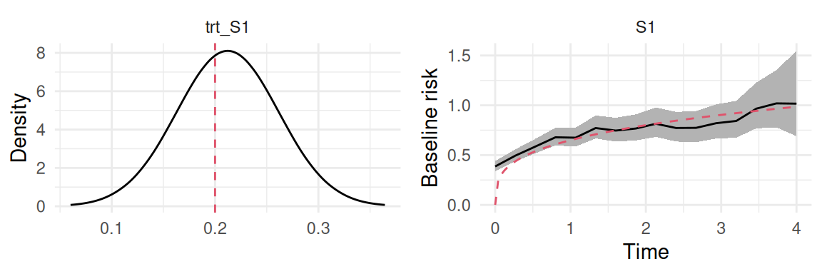
Finally, we can have a look at the standard deviation of the Besag random effect:
plot(M_bs)$Covariances[[1]] + theme(legend.position = "")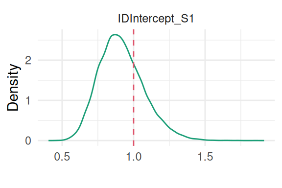
We can also directly display the random effect estimated on the map, and compare to the true values. The summary statistics over the posterior distribution of the random effect for each department is available in the summary.random argument of the fitted object:
fit <- M_bs$summary.random$IDIntercept_S1$mean
ggarrange(ggplot() + geom_sf(data=fr1, aes(fill=fit)) + ggtitle("Fitted"),
ggplot() + geom_sf(data=fr1, aes(fill=s.besag)) + ggtitle("True"))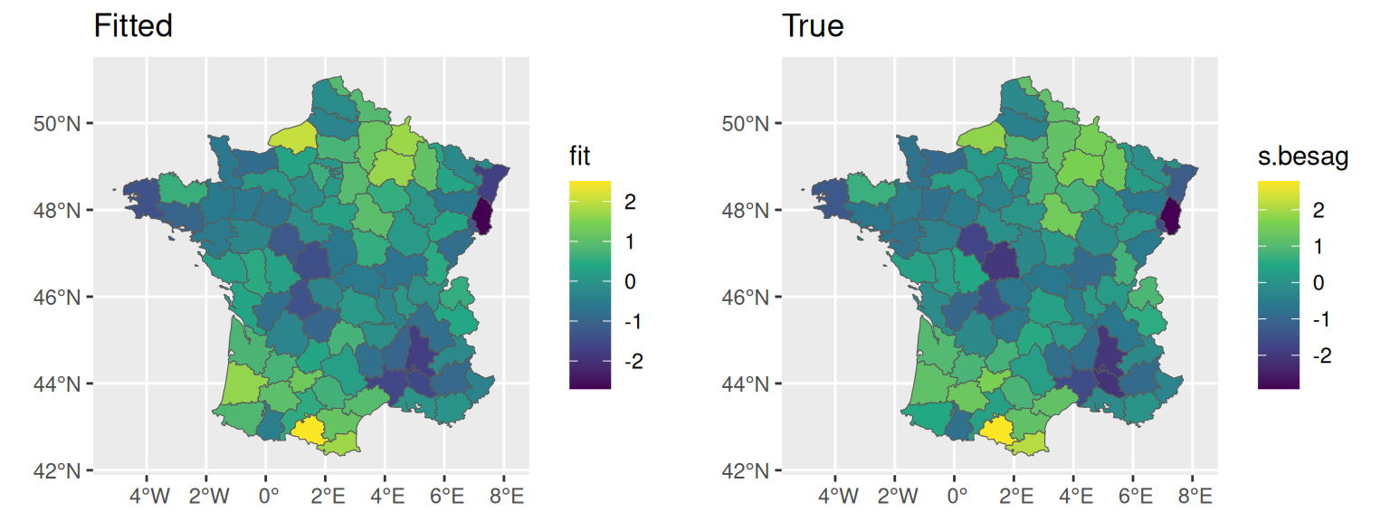
and since we have summary statistics, we can also for example display the standard deviations of the spatial random effect:
fitsd <- M_bs$summary.random$IDIntercept_S1$sd
ggarrange(ggplot() + geom_sf(data=fr1, aes(fill=fit)) + ggtitle("Fitted"),
          ggplot() + geom_sf(data=fr1, aes(fill=fitsd)) +
          ggtitle("Standard deviations"))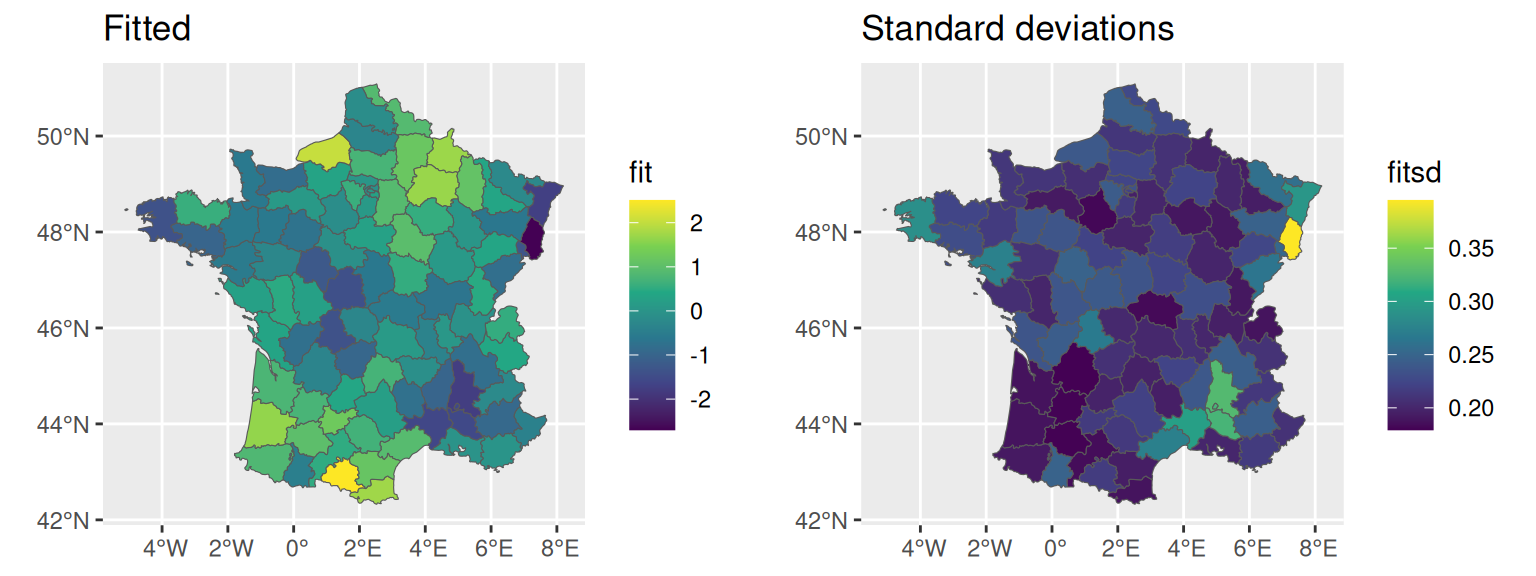
Although the spatially structured random effect is not directly handled by INLAjoint, we can still use the predict function to predict the outcome for new individuals or specific scenarios. For example here, we consider two new individuals, one coming from the department with the highest average risk while the second individual comes from the department with the lowest risk:
minS <- M_bs$summary.random$IDIntercept_S1$ID[which.min(
  M_bs$summary.random$IDIntercept_S1$mean)]
maxS <- M_bs$summary.random$IDIntercept_S1$ID[which.max(
  M_bs$summary.random$IDIntercept_S1$mean)]
ND <- datSbesag[c(which(datSbesag$id_s%in%c(minS))[1],
                which(datSbesag$id_s%in%c(maxS))[1]),]
ND$eventTimes <- 0;ND$eventIndic <- 0
ND$id_s <- ifelse(ND$id_s==minS, "Department with lowest risk",
                  "Department with highest risk");ND
id eventTimes eventIndic trt id_s
51 51 0 0 0 Department with lowest risk
31 31 0 0 0 Department with highest riskThe trick for the predict function to account for the spatially structured random effect is to pre-sample realisations of this random effect for each of the two scenarios (i.e., here our two departments), which can be done with the function inla.posterior.sample:
NsampleHY <- 20
NsampleFE <- 20
Besag_samples <- sapply(inla.posterior.sample(NsampleHY*NsampleFE, M_bs,
  selection=list("IDIntercept_S1"=c(minS, maxS))), function(x) x$latent)
if(minS>maxS) Besag_samples <- Besag_samples[2:1,]
rownames(Besag_samples) <- unique(ND$id_s)
summary(t(Besag_samples))
Department with lowest risk Department with highest risk
Min. :-3.575 Min. :1.872
1st Qu.:-2.945 1st Qu.:2.351
Median :-2.669 Median :2.495
Mean :-2.670 Mean :2.498
3rd Qu.:-2.401 3rd Qu.:2.641
Max. :-1.756 Max. :3.079 We can see how the sampled realisations of the random effect are very different on average, now we can call the predict function and we use the argument set.samples to indicate that we provide pre-sampled values of the spatial random effect:
P <- predict(M_bs, ND, horizon=3, survival=T,
             set.samples=list("IDIntercept_S1"=Besag_samples))
and we can plot the survival probability over time for these two departments:
ggplot(P$PredS, aes(x=eventTimes, y=Surv_quant0.5)) + ylim(0,1) +
  geom_ribbon(aes(ymin=Surv_quant0.025, ymax=Surv_quant0.975), alpha=0.1)+
  geom_line() + theme_minimal() + facet_wrap(~id_s) + xlab("Time") +
  ylab("Survival probability")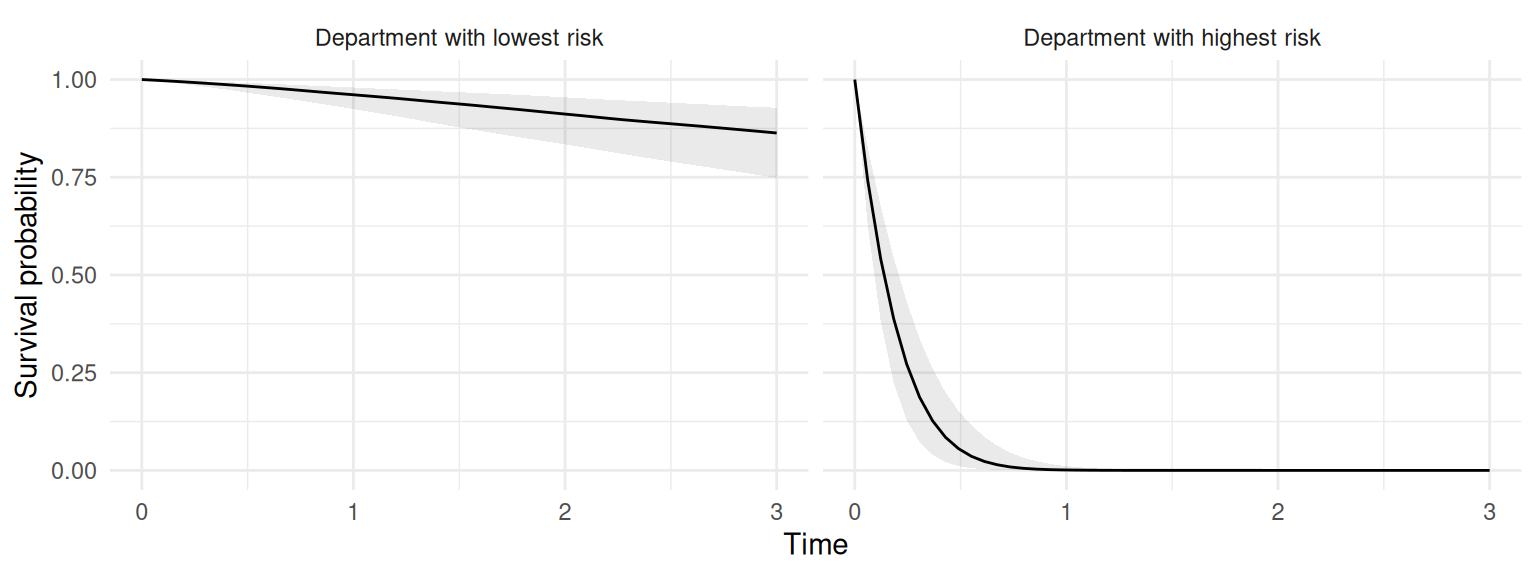
Here we can see very different survival probabilities over time for these two individuals, which is only due to their geographical position on the map since we assume both are from the same treatment group (which is the only covariate included in this model).
If we did not provide pre-sampled values of the random effect, the predict function assume the individual comes from a new draw from the marginal posterior of the random effect which means this individual may come from any department, we don’t know which one:
ND2 <- ND[1,]
ND2$id_s <- "Undefined location"
P <- predict(M_bs, ND2, horizon=3, survival=T)
ggplot(P$PredS, aes(x=eventTimes, y=Surv_quant0.5)) + ylim(0,1) +
  geom_ribbon(aes(ymin=Surv_quant0.025, ymax=Surv_quant0.975), alpha=0.1)+
  geom_line() + theme_minimal() + facet_wrap(~id_s) + xlab("Time") +
  ylab("Survival probability")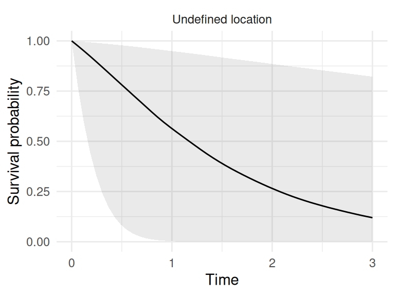
More generally, when we want to predict for a random effect category from which we already learned (spatial or not), using set.sample allows us to consider a new individual belonging to a known category of the random effect, by computing the predictions based on pre-sampled conditional posteriors of the relevant random effect.
The Besag model assumes that all unexplained variation in the outcome is spatially structured. The unexplained variation may however be a mixture of spatial clustering (where neighboring areas share common risk factors) and unstructured heterogeneity which represents area-specific variability that is independent of neighbors. The Besag-York-Mollié (BYM) model (Besag et al. (1991)) was proposed to enhance the modeling of spatial data by explicitly separating the latent variability into spatially structured random effect through an ICAR prior and an unstructured random effect to account for the residual variability that is not explained by the spatial structure, often modeled using a normal distribution with zero mean and a precision parameter. It allows for the identification of areas with elevated or reduced risk while accounting for both spatial dependencies and residual variability.
In its original formulation, the BYM model lacks the interpretable variance of the scaled Besag model. We thus use the scaled BYM model, hereafter named as the BYM2 model, as proposed in Riebler et al. (2016). Thus, the BYM2 model for the spatial effect is defined as \[ b_s = \frac{1}{\sqrt{\tau}_b} (\sqrt{\phi} \cdot u_s + \sqrt{1-\phi}\cdot v_s) \] where \(u_s=\{u_1,\ldots,u_m\}\) follows a scaled ICAR model (see Section 5.1), and \(v_s\) are independent and identically distributed standard Gaussian variables. Because \(u\) follows a scaled Besag model, and has a unit variance, the spatial effect is now a weighted average of \(u\) and \(v\), where \(\phi\) is the weight and can be interpreted as the proportion of the spatial effect \(b\) that is structured in space. Furthermore, we can also interpret \(\sigma_b^2=1/\tau_b\) as a marginal variance.
In addition, as proposed in Riebler et al. (2016), we consider the Penalized Complexity (PC) prior on both model parameters. The prior for these parameters is specified considering the two following probability statements, \(P(\phi \geq u_\phi)=\alpha_\phi\) and \(P(\sigma_b \geq \sigma_0)=\alpha_\sigma\), where \(u_\phi\) and \(\sigma_0\) are reference values for these parameters and \(\alpha_\phi\) and \(\alpha_\sigma\) are tail probability values (see Section 1.1.2.1).
Following the previous example, we can add the unstructured component to have the BYM2 model within a survival model. The model definition remains as \[\lambda_{i}(t)=\lambda_{0}(t)\ \textrm{exp}\left(\gamma\cdot trt_i + b_{s(i)}\right)\] but \(b_{s(i)}\) now follows a BYM2 model.
We can simulate from this model:
phi <- 0.5
s.IID <- rnorm(n.areas)
s.bym <- (sqrt(phi)*s.besag + sqrt(1-phi)*s.IID)
eventTimes <- (-(log(u))/(baseScale*exp(trt*gamma_1 +
                                        s.bym[id_s])))^(1/baseShape)
eventIndic <- as.numeric(eventTimes<followup)
eventTimes <- pmin(eventTimes, followup)
datSbym <- data.frame(id=1:n, eventTimes, eventIndic, trt, id_s)
summary(datSbym)[,-1]
eventTimes eventIndic trt id_s
Min. :0.001399 Min. :0.0000 Min. :0.000 Min. : 1.00
1st Qu.:0.423920 1st Qu.:1.0000 1st Qu.:0.000 1st Qu.:23.00
Median :1.017893 Median :1.0000 Median :0.000 Median :47.00
Mean :1.481652 Mean :0.8775 Mean :0.499 Mean :47.03
3rd Qu.:2.220313 3rd Qu.:1.0000 3rd Qu.:1.000 3rd Qu.:70.00
Max. :4.000000 Max. :1.0000 Max. :1.000 Max. :94.00 Now the random effect’s value s.bym is a combination of the previously simulated random effect s.besag and an additional unstructured random effect s.IID.
The model fit is similar to Besag, except that we have to define the model as bym2 and we don’t need to include scale.model=TRUE since the model is already scaled by definition.
M_bym0 <- joint(formSurv = list(inla.surv(eventTimes,
                                          eventIndic) ~ trt + (1|id_s)),
               dataSurv=datSbym, id="id_s", run=F)
M_bym0$.args$data$IDbym_S1 <- M_bym0$.args$data$IDIntercept_S1
M_bym0$.args$formula <- as.formula(paste(c("Yjoint ~ -1 ",
  attr(terms(M_bs0$.args$formula), which = "term.labels")[1:3],
  "f(IDbym_S1, model='bym2', graph=Graph)"), collapse="+"))
M_bym <- joint.run(M_bym0)
summary(M_bym)
Survival outcome
                           mean     sd 0.025quant 0.5quant 0.975quant
Baseline risk (variance) 0.0616 0.0317     0.0212   0.0546     0.1435
trt                      0.2029 0.0497     0.1054   0.2029     0.3004

Spatial effect
                         mean     sd 0.025quant 0.5quant 0.975quant
Phi for IDbym_S1       0.6417 0.1730     0.2726   0.6604     0.9172
Precision for IDbym_S1 0.9688 0.1875     0.6482   0.9524     1.3833

log marginal-likelihood (integration)    log marginal-likelihood (Gaussian)
                            -6297.313                             -6296.098

Deviance Information Criterion:  12491.08
Widely applicable Bayesian information criterion:  12488.84
Computation time: 2.63 seconds
We can see the summary includes both the precision of the spatial random effect and the \(\phi\) parameter that weights the proportion of the department level variability that is structured in space, with the unstructured component.
The spatial random effect value (which is the sum of the structured and unstructured) is available in summary.random, which we can directly plot:
fitted <- M_bym$summary.random$IDbym_S1$mean[1:94]
ggarrange(ggplot()+geom_sf(data=fr1,aes(fill=fitted))+ggtitle("Fitted"),
          ggplot()+geom_sf(data=fr1,aes(fill=s.bym))+ggtitle("True"))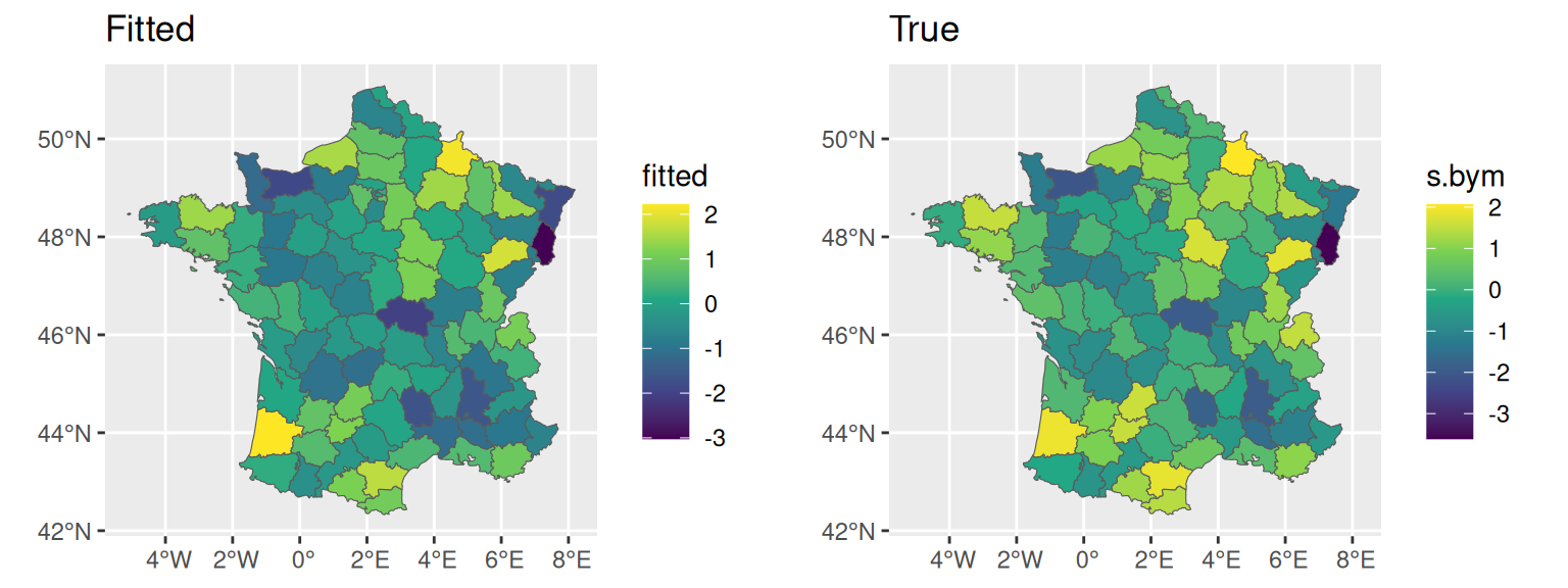
Of note, the size of the random effect as displayed in summary.random is twice larger than the Besag which was size 94 (i.e., one per department). For the BYM model, the first 94 values are the sum of the structured and unstructured random effect and the 94 remaining values corresponds to the unstructured random effect only.
Now we show an example of a spatial longitudinal model based on the BYM2 random effect. Let’s consider the following model: \[\textrm{E}[Y_{i}(t)]=\beta_0 + b_{i0} + \beta_1\cdot t + \beta_2\cdot trt_i + \beta_3\cdot trt_i\cdot t + b_{s(i)}\]
The model includes an individual iid random intercept in addition to the spatially structured random effect. We can simulate from this model, using the same simulated spatial values as in the previous example, therefore we only need to simulate repeated measurements of a marker that depend on this spatial random effect:
b_0=2 # intercept
b_1=-1 # slope
b_2=-2 # trt
b_3=1 # trt x slope
b_e=1 # residual error
b_intSD=0.5 # random intercept standard deviation
mestime=seq(0, 5, 1) # measurement times
n_i <- length(mestime)
time=rep(mestime, n) # time column
id<-rep(1:n, each=n_i) # individual id
b_int <- rep(rnorm(n, mean=0, sd=b_intSD), each=n_i) # random intercept
trtY=rep(trt, each=n_i) # binary trt covariate
linPred <- b_0 + b_int + b_1*time + b_2*trtY + b_3*trtY*time +
                                    rep(s.bym[id_s], each=n_i) # spatial
Y <- rnorm(n_i*n, linPred, b_e) # observed outcome
datLbym <- data.frame(id, time, Y, trt=trtY,
                     id_s=rep(id_s, each=n_i))
str(datLbym) # longitudinal dataset
'data.frame': 12000 obs. of 5 variables:
$ id : int 1 1 1 1 1 1 2 2 2 2 ...
$ time: num 0 1 2 3 4 5 0 1 2 3 ...
$ Y : num -0.575 1.61 -1.301 -0.641 -1.507 ...
$ trt : int 0 0 0 0 0 0 1 1 1 1 ...
$ id_s: int 64 64 64 64 64 64 4 4 4 4 ...In order to fit this model, we use a different strategy as with the survival model because we now want our iid random effect and we need to add the spatial one (i.e., we need to setup the spatial id in addition to the individual id). First, we setup the model ignoring the spatial random effect, but we use the argument run=FALSE to be able to add the spatially structured random effect before running INLA:
M_bymL0 <- joint(formLong = Y ~ time * trt + (1|id),
                 dataLong=datLbym, id = "id", timeVar = "time", run=F)

M_bymL0$.args$data$IDbym_L1 <- datLbym$id_s # add spatial effect
M_bymL0$.args$formula <- as.formula(paste(c("Yjoint ~ -1 ",
          attr(terms(M_bymL0$.args$formula), which = "term.labels"),
          "f(IDbym_L1, model='bym2', graph=Graph)"), collapse="+"))
M_bymL <- joint.run(M_bymL0)
summary(M_bymL)
Longitudinal outcome (gaussian)
mean sd 0.025quant 0.5quant 0.975quant
Intercept 2.0432 0.0732 1.8968 2.0432 2.1896
time -0.9979 0.0076 -1.0127 -0.9979 -0.9830
trt -2.0058 0.0401 -2.0844 -2.0058 -1.9273
time:trt 1.0033 0.0107 0.9823 1.0033 1.0243
Res. err. (variance) 1.0049 0.0141 0.9773 1.0050 1.0326
Random effects variance-covariance (L1)
mean sd 0.025quant 0.5quant 0.975quant
Intercept 0.2493 0.0136 0.2231 0.2493 0.2763
Spatial effect
mean sd 0.025quant 0.5quant 0.975quant
Phi for IDbym_L1 0.8072 0.1412 0.4531 0.8428 0.9803
Precision for IDbym_L1 0.8102 0.1517 0.6033 0.7840 1.1882
log marginal-likelihood (integration) log marginal-likelihood (Gaussian)
-18151.08 -18148.85
Deviance Information Criterion: 35355.14
Widely applicable Bayesian information criterion: 35399.24
Computation time: 2.85 secondsThe model seems to fit well the data and recover true values used for data generation, we can compare the fitted random effect posterior to the true values:
fitT <- M_bymL$summary.random$IDbym_L1$mean[1:94]
ggarrange(ggplot()+geom_sf(data=fr1,aes(fill=fitT))+ggtitle("Fitted"),
          ggplot()+geom_sf(data=fr1,aes(fill=s.bym))+ggtitle("True"))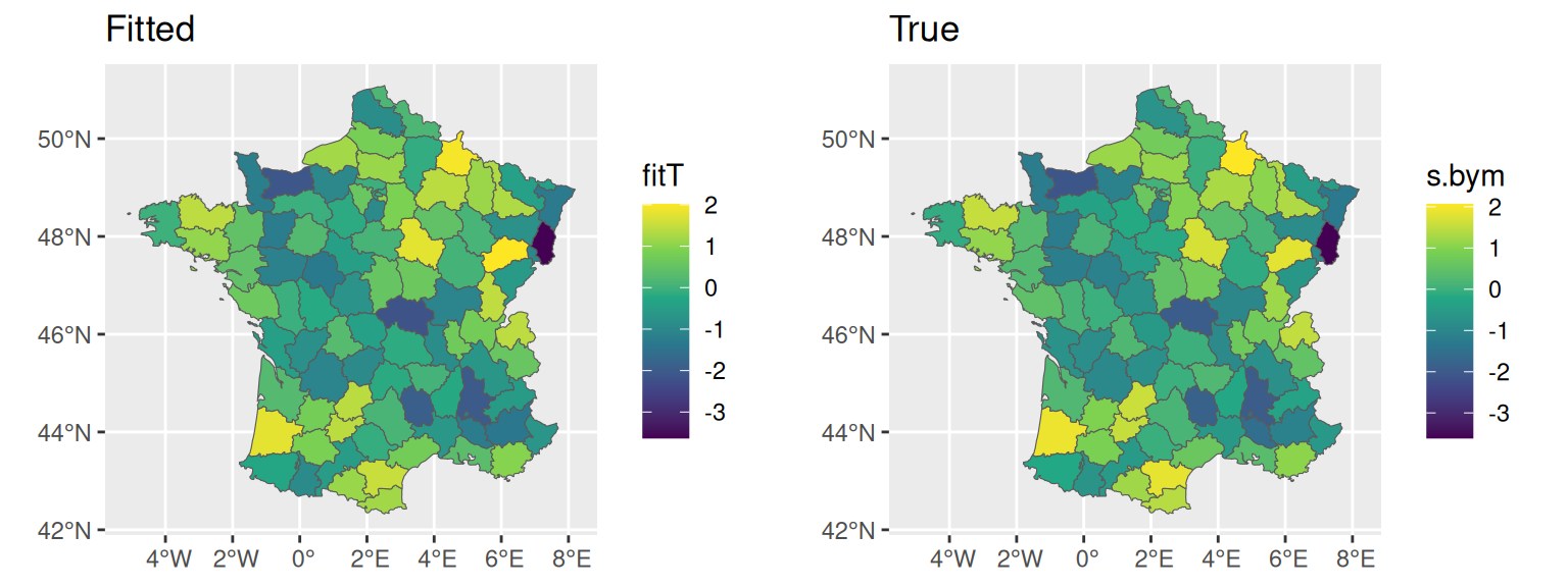
Now we have both survival and longitudinal submodels linked by the use of the same spatial random effect. We can therefore fit a joint model to fit these two outcomes simultaneously.
We can consider the following joint model: \[\begin{equation*} \left\{ \begin{array}{lc} \textrm{E}[Y_{i}(t)]= \beta_0 + b_{i0} + \beta_1\cdot t + \beta_2\cdot trt_i + \beta_3\cdot trt_i\cdot t + b_{s(i)}\\ \lambda_i(t)=\lambda_0(t)\exp\left(\gamma_1\cdot \textrm{trt}_i + \gamma_2\cdot b_{s(i)}\right) \end{array} \right. \end{equation*}\]
Note how the BYM2 is included in the longitudinal submodel and scaled by \(\gamma_2\) in the survival submodel (we assume \(\gamma_2=1\) for simplicity in the data simulation but this parameter is estimated in the model, as shown below). This model can be fitted by combining the survival and longitudinal submodels in the call of the joint() function. Since we have an iid random intercept in the longitudinal dataset that is not shared and a spatially structured random effect shared between the two submodels, we can take advantage of INLAjoint to build the model with each id level, then we can just copy the spatially structured shared random effect id in the model that includes the iid random effect:
# only iid random intercept in longitudinal submodel
M_JMbym0 <- joint(formSurv = list(inla.surv(eventTimes,eventIndic) ~ trt),
                 formLong = Y ~ time * trt + (1|id),
                 dataSurv=datSbym, dataLong=datLbym,
                 id = "id", timeVar = "time", assoc="", run=F)
# fake model to construct the shared spatial id
M_JMbym1 <- joint(formSurv = list(inla.surv(eventTimes,eventIndic) ~ trt),
                  formLong = Y ~ time * trt + (1|id_s),
                  dataSurv=datSbym, dataLong=datLbym,
                  id = "id_s", timeVar = "time", assoc="SRE_ind",
                  reorder=F, run=F)
The reorder option prevents the automatic reordering of the data according to id, which avoids mismatchs here since the spatial id is not ordered. Now we can extract the spatial id and add it to the model including the iid random effect, using a different name to identify it clearly:
M_JMbym0$.args$data$IDbym_L1 <- M_JMbym1$.args$data$IDIntercept_L1
M_JMbym0$.args$data$SRE_bym_L1_S1 <-
  M_JMbym1$.args$data$SRE_Intercept_L1_S1
Finally, we modify the formula to add the shared and scaled BYM2 random effect using the new ids we just added to the internal data. We also add the name of the new random effect in the argument REstruc which informs about random effects structure for internal computations:
M_JMbym0$.args$formula <- as.formula(paste(c("Yjoint ~ -1 ",
  attr(terms(M_JMbym0$.args$formula), which = "term.labels"),
  "f(IDbym_L1, model='bym2', graph=Graph) +
   f(SRE_bym_L1_S1, copy='IDbym_L1', fixed=F)"), collapse="+"))
M_JMbym0$REstruc <- c(M_JMbym0$REstruc, "IDbym_L1")
In the new formula, we first setup the random effect in the longitudinal part with the corresponding id IDbym_L1, then we copy and scale this BYM2 random effect in the survival model with the id SRE_bym_L1_S1. Note that setting fixed=TRUE would remove the scaling parameter (which is not necessary here since we simulated with \(\gamma_2=1\) but in other applications it could important to scale the shared random effect between different outcomes). Since the model is defined to have a scaling parameter in the survival submodel, here we take advantage of the INLAjoint structure and we define the random effect in the longitudinal and scale it in the survival but we could also move the scaling parameter to the longitudinal submodel instead. Now we can run INLA to fit the model:
M_JMbym <- joint.run(M_JMbym0)
summary(M_JMbym)
Longitudinal outcome (gaussian)
mean sd 0.025quant 0.5quant 0.975quant
Intercept_L1 2.0433 0.0686 1.9054 2.0433 2.1813
time_L1 -0.9979 0.0076 -1.0127 -0.9979 -0.9830
trt_L1 -2.0071 0.0399 -2.0854 -2.0071 -1.9288
time:trt_L1 1.0033 0.0107 0.9823 1.0033 1.0243
Res. err. (variance) 1.0048 0.0141 0.9765 1.0051 1.0319
Random effects variance-covariance (L1)
mean sd 0.025quant 0.5quant 0.975quant
Intercept_L1 0.2498 0.0136 0.2236 0.2497 0.2769
Spatial effect
mean sd 0.025quant 0.5quant 0.975quant
Phi for IDbym_L1 0.6478 0.1975 0.1966 0.6847 0.9219
Precision for IDbym_L1 0.8242 0.1566 0.5670 0.8071 1.1813
Survival outcome
mean sd 0.025quant 0.5quant 0.975quant
Baseline risk (variance)_S1 0.0580 0.0303 0.0184 0.0517 0.1352
trt_S1 0.2179 0.0483 0.1231 0.2179 0.3127
Association longitudinal - survival
mean sd 0.025quant 0.5quant 0.975quant
SRE_bym_L1_S1 0.9465 0.0336 0.8822 0.9458 1.0145
log marginal-likelihood (integration) log marginal-likelihood (Gaussian)
-24388.47 -24384.45
Deviance Information Criterion: 47775.59
Widely applicable Bayesian information criterion: 47818.9
Computation time: 5.65 secondsThe fitted model includes both longitudinal and survival parts, as well as the summary statistics over the spatial random effect. As expected, the scaling parameter for the shared spatial random effect SRE_bym_L1_S1 includes the true value (1) in the credible interval. We can display the posterior of the BYM random effect:
fitL <- M_JMbym$summary.random$IDbym_L1$mean[1:94] # fitted

ggarrange(ggplot()+geom_sf(data=fr1, aes(fill=fitL))+
            ggtitle("Fitted"),
          ggplot()+geom_sf(data=fr1, aes(fill=s.bym))+
            ggtitle("True"))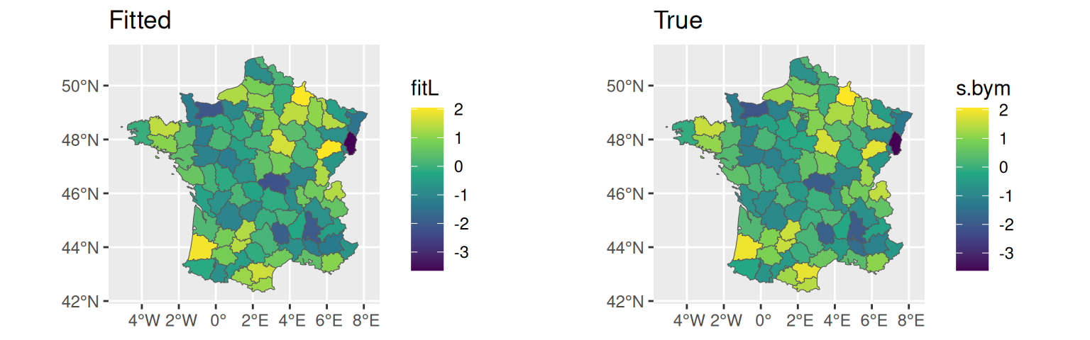
Of note, we are not limited to associations where only the spatial random effect is shared and scaled. All the associations described in Chapter 4 can in theory include spatial random effects such that if we used association assoc="CV" in our model setup, we would share the entire linear predictor including the spatial random effect.
Let’s illustrate predictions by considering two individuals coming from two specific departments:
NDbym <- datLbym[c(1,1),]
NDbym$Y <- NA
NDbym$id_s <- c(1,8) # select two departments
NDbym$id <- c(1,2)
We need to sample from the conditional posterior of the random effect for these two departments to account for the spatial effect in the predictions (while the iid random effect is assuming the two individuals as new draws from the marginal posterior of the iid random effect, since we do not provide any longitudinal outcome measurement to update the marginal posterior distribution of this random effect):
NsampleHY <- 20
NsampleFE <- 20
Besag_samples <- sapply(inla.posterior.sample(NsampleHY*NsampleFE,M_JMbym,
  selection=list("IDbym_L1"=NDbym$id_s)), function(x) x$latent)
P <- predict(M_JMbym, NDbym, horizon=3, survival=T,
             set.samples=list("IDbym_L1"=Besag_samples))

ggarrange(ggplot(P$PredL, aes(x=time, y=quant0.5)) +
  geom_ribbon(aes(ymin=quant0.025, ymax=quant0.975), alpha=0.1)+
  geom_line() + theme_minimal() + facet_wrap(~id) + xlab("Time") +
  ylab("Longitudinal marker"),
ggplot(P$PredS, aes(x=time, y=Surv_quant0.5)) + ylim(0,1) +
  geom_ribbon(aes(ymin=Surv_quant0.025, ymax=Surv_quant0.975), alpha=0.1)+
  geom_line() + theme_minimal() + facet_wrap(~id) + xlab("Time") +
  ylab("Survival probability"), nrow=2)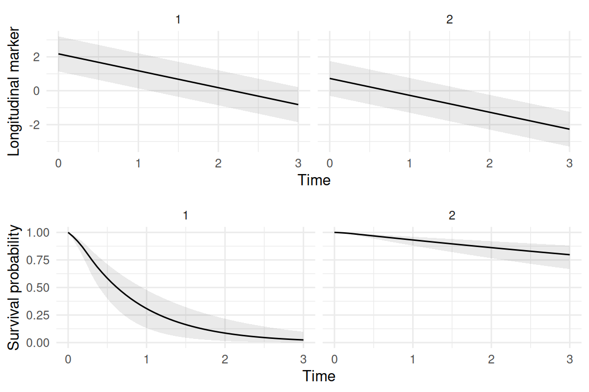
We can see how both the longitudinal and survival trajectories differ, which only results from the differences at the spatial level (different departments).
The previous sections focused on areal data, where observations are aggregated over areas like departments, and spatial correlation is modeled through a discrete neighborhood graph. We now introduce point reference data, where each observation is associated with a specific set of coordinates (e.g., longitude and latitude). The goal is now to model the random effect as a continuously varying spatial field across the entire domain.
Therefore, we consider a continuous-spatial domain stochastic process where it is assumed that at any location \(s\) we can have a random variable \(b_s\) that varies smoothly over the spatial domain. Considering the locations \(s\) and \(s'\) not far from each other, we suppose that \(b_s\) and \(b_{s'}\) are similar, or highly correlated.
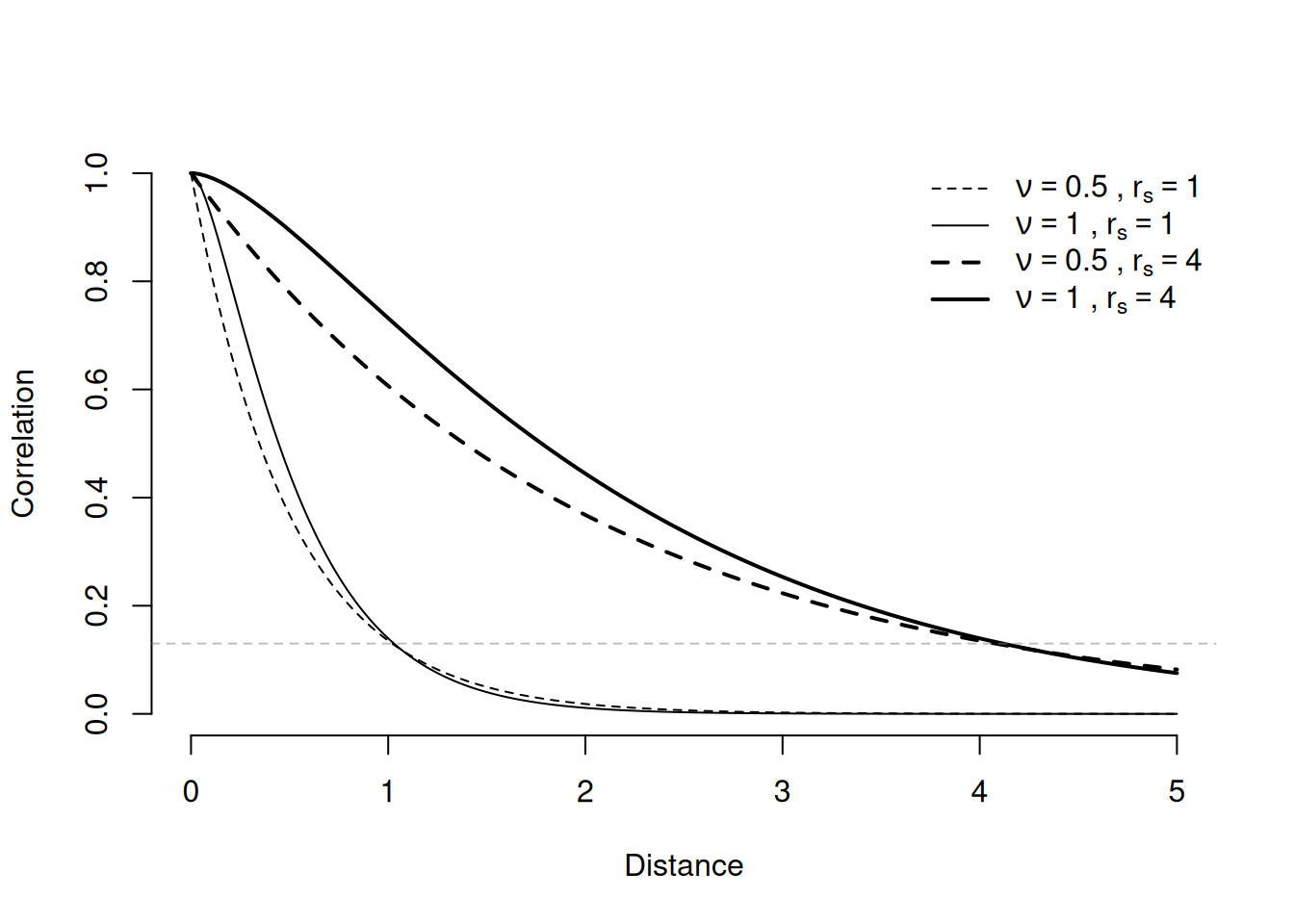
One approach consists in considering a model for the difference between, \(b_s\) and \(b_{s'}\) (Matheron (1963)). Equivalently, we can consider a correlation function for the process \(b\) so that the correlation between \(b_s\) and \(b_{s'}\) decreases as the distance between \(s\) and \(s'\) increases. The most used model for that is the Matérn correlation function (Matérn (1960)), which is a function of the distance \(h\) between two locations, and two hyperparameters, denoted as C(\(h\),\(r_s\),\(\nu\)), and can be written as \[ \textrm{c}(h,r_s,\nu) = \frac{2^{1-\nu}}{\Gamma(\nu)} (2 \cdot \nu \cdot h/r_s) \cdot \mathsf{K}(\nu, 2\cdot \nu \cdot h/r_s) \] where \(\nu\) is a smoothness parameter, \(\mathsf{K}\) is the modified Bessel function of second kind, and \(r_s\) is a (practical) correlation range, so that c(\(h=r_s\))\(\approx 0.13\). Usually the data analysis focus on estimating the range parameter because it gives the direct interpretation on how far to go so that the correlation is small. We can see in the next figure the correlation as a function of the distance for some values of \(\nu\) and \(r_s\).
There is a direct link between modeling the variation between \(b_{s}\) and \(b_{s'}\), and the Stochastic Partial Differential Equation approach, which has been considered in the spatial statistics literature (Whittle (1954)). This direct link is that the solution of a linear SPDE is a random field with Matérn covariance and have received more attention in spatial statistics after the work by Lindgren et al. (2011). In this work, the Finite Element Method (FEM) was proposed as a practical way to solve the linear SPDE. The proposed method using FEM provide that the solution at a set of mesh nodes is a GMRF.
The precision matrix for \(\nu=1\) (the most common value) at the mesh nodes is \[ Q = \tau^2(\kappa^4 \cdot C + 2\kappa^2 \cdot G + G^{2}) \] where the sparse matrices \(C\), \(G\) and \(G^{2}\) are derived from the FEM method proposed in Lindgren et al. (2011), \(\kappa = 1/r_s\) is a scale parameter, \(\tau^2\) is a conditional precision parameter and we will use \(\sigma_u^2=\frac{1}{2\pi \cdot \tau^2 \cdot \kappa^2}\) as the marginal variance parameter. See Lindgren & Rue (2015) for additional details.
This offers several computational advantages over using the covariance for model fitting, including its ability to handle large datasets, making it a powerful tool for modern spatial analysis. Therefore, to apply it in practice we have to build a mesh, which is made up from a set of triangles covering the map. The spatial effect is then modeled at the mesh nodes and is projected onto the observation locations.
This approach can be viewed as a case of a generalized mixed models where the spatial effect has a design matrix. We can write the linear predictor as \[ \eta_i = X_i^\top\beta + A_ib_{s_0} \] where \(X_i\) includes the covariates for individual \(i\), \(\beta\) is the vector of fixed effects, \(A_i\) is the \(\text{i}^{\text{th}}\) row of the projector matrix (i.e., the spatial random effect design matrix) to project the spatial effect \(b_{s_0}\) that is modeled at the mesh nodes \(s_0\).
In order to illustrate the SPDE modeling approach, we now consider observations can be observed at any precise location on the map, as defined by coordinates. Let’s consider a function to simulate locations:
rpoint <- function(n, map, m.loc, s.loc = c(5, 5)) {
  bb <- matrix(st_bbox(map), 2)
  out <- matrix(NA, n, 2)
  n0 <- 0
  repeat{
    if(missing(m.loc)) {
      xy0 <- st_as_sf(
        data.frame(x = runif(n, bb[1, 1], bb[1, 2]),
                   y = runif(n, bb[2, 1], bb[2, 2])),
        coords = 1:2, crs = st_crs(map))
    } else {
      x0 <- rnorm(n, m.loc[1], s.loc[1])
      y0 <- rnorm(n, m.loc[2], s.loc[2])
      xy0 <- st_as_sf(
        data.frame(x = x0, y = y0),
        coords = 1:2, crs = st_crs(map))
    }
    id0 <- unlist(st_contains(map, xy0))
    nn <- min(length(id0), n-n0)
    if(nn>0) {
      out[n0 + 1:nn, ] <- st_coordinates(xy0[sample(id0, nn), ])
      n0 <- n0 + nn
    }
    if(n0>=n)
      break
  }
  return(out)
}
We can simulate locations for a sample of observed data:
xy <- rpoint(n, fr1, m.loc = c(-2, 50), c(3, 3))
library(sf)
xy_sf <- st_as_sf(data.frame(xy),
                  coords = 1:2, crs=st_crs(fr1))
ggplot() + theme_minimal() +
  geom_sf(data = fr1) +
  geom_sf(data = xy_sf)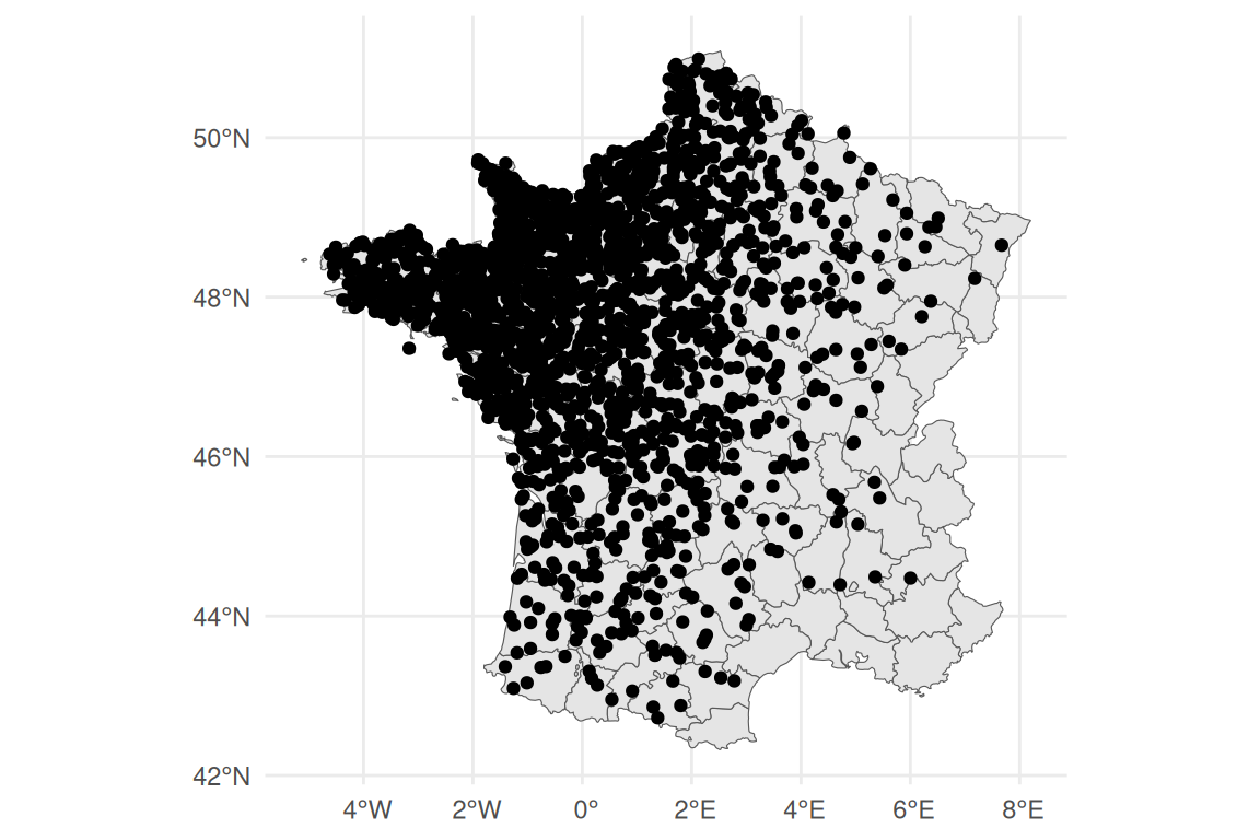
Here we have defined non-homogeneously distributed observations locations to better illustrate the properties of the SPDE model, particularly in terms of uncertainty quantification, such that we have a lot of observations in the North-West and less information in the South-East. Now we need to define a mesh that will decompose space in triangles, where each node is a level of the spatial random effect. Then it is possible to interpolate any point on the map based on at most the 3 corresponding nodes of the triangle where we want to interpolate (2 when the point is aligned with two mesh nodes). Importantly, to avoid “border effect” which can lead to biased estimation of the spatial effect near borders, we extend the mesh beyond the borders to ensure smooth estimates even in the border (without this extension, the model interprets borders as impassable walls, which leads to undesirable properties since most of the time, borders are only defining the limits of the area of interest but should not afffect the distribution of the data of interest). The R package fmesher (Lindgren (2025)) is used to build the mesh:
library(fmesher)
bb <- matrix(st_bbox(fr1), 2)
r2 <- apply(bb, 1, diff)
rr <- mean(r2)
the_crs <- st_crs(fr1)
mesh <- fm_mesh_2d(boundary = fr1,
  max.edge = rr/c(30, 10), # inside => size of map/30 / outside 10
  offset = rr/c(10, 5), # extension around the map
  cutoff = rr/60, # avoid small triangles
  crs = the_crs)
ggplot() + geom_fm(data = mesh, fill = "white", color = "black") +
  theme_void()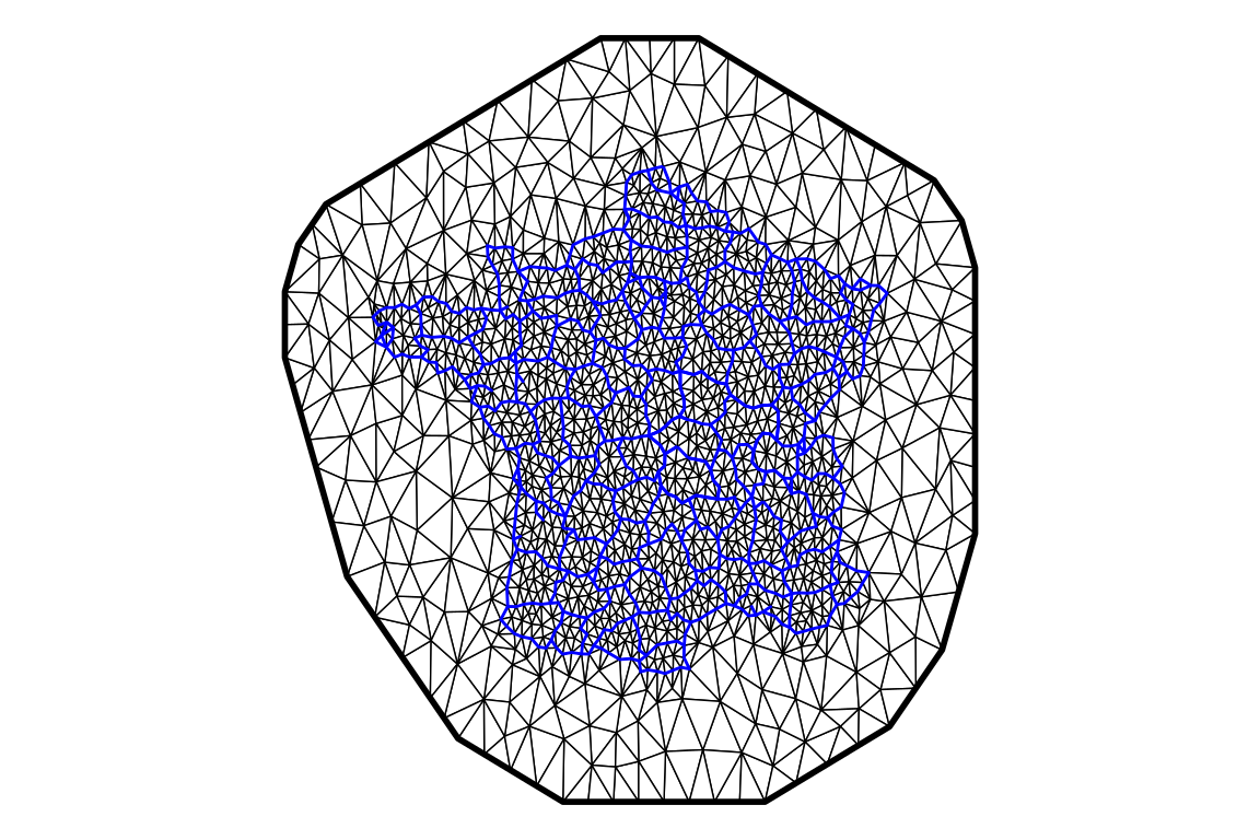
The function fm_mesh_2d is used to create the mesh. The size of triangles inside the area of interest is given as a fraction of the map size, here 1/30 and the size of triangles outside the area of interest to avoid border effects is 1/10 of the map size (we don’t need fine resolution in this area which is not of interest). The size of the extension beyond the borders of interest is given by offset, when sufficiently large it has no influence other that increasing the computational burder, it is therefore usually kept within a reasonable range to eliminate border effect without adding too much computations. Finally, the argument cutoff is setting a limit to avoid too small triangles which could result in numerical instabilities.
Now we can project the simulated locations on the mesh with the function fm_evaluator:
# projector from mesh nodes to locations
A <- fm_evaluator(mesh = mesh, loc = xy)
The SPDE model is built with the R-INLA function inla.spde2.pcmatern:
# Define the SPDE model
spde <- inla.spde2.pcmatern(
  mesh = mesh,
  alpha = 2,
  prior.range = c(rr/50, 0.05), # P(range < r0) = 0.05
  prior.sigma = c(2, 0.05),     # P(sigma < s0) = 0.05
  constr = TRUE
)
The prior distributions related to the SPDE model are defined here, the use of PC priors allows for an intuitive interpretation of these priors and an easy setup of vague priors. The prior on range is defined such that \(P(r_s<r_0)=\alpha_{r}\), meaning that the probability that the range is lower that \(r_0\) is \(\alpha_{r}\). Similarly, for the \(\sigma\) parameter (i.e., standard deviation of the spatial random effect), the probability that the standard deviation is lower than \(\sigma_0\) is \(\alpha_\sigma\): \(P(\sigma<\sigma_0)=\alpha_\sigma\).
The hyperparameters of the SPDE indeed include the range and the variability of the effect, we can define them as follows:
s.range <- rr/5 # parameter: spatial practical range
tau.SPDE <- 1 # parameter: spatial precision
Q.spatial <- inla.spde2.precision(
  spde = spde,
  theta = log(c(s.range, 1/sqrt(tau.SPDE)))
)
Here, Q.spatial is the precision matrix for the SPDE model built at the mesh. We can use it to simulate the spatial random effect at the mesh nodes, with the inla.qsample function given Q.spatial. This is then projected to the individual locations, to be used as the spatial random effect for each individual to illustrate the model application:
spatialREmesh <- inla.qsample(n = 1, Q = Q.spatial, seed = 1)
s.sample <- drop(A$proj$A %*% spatialREmesh)
Now that we have observations of the spatial random effect, we can simulate time-to-event observations as well as repeated measurements of a longitudinal marker, such that we have a joint model with a shared spatial random effect, as described in the following model: \[\begin{equation*} \left\{ \begin{array}{lc} \textrm{E}[Y_{i}(t)]= \beta_0 + b_{i0} + \beta_1\cdot t + \beta_2\cdot trt_i + \beta_3\cdot trt_i\cdot t + b_{s(i)} \\ \lambda_i(t)=\lambda_0(t)\exp\left(\gamma_1\cdot trt_i + \gamma_2\cdot b_{s(i)}\right) \end{array} \right. \end{equation*}\] where \(b_{s(i)}=A_i b_{s_0}\) is the spatial random effect at the location of individual \(i\) while \(b_{i0}\) is an individual iid random effect.
We can simulate longitudinal data conditional on this random effect:
# generation of longitudinal data conditional on SPDE (s.sample)
linPred <- b_0 + b_int + b_1*time + b_2*trt + b_3*trt*time +
  rep(s.sample, each = n_i) # spatial random effect
Y <- rnorm(n_i*n, linPred, b_e) # observed outcome
longDat <- data.frame(id, time, Y, trt = trt)
str(longDat) # longitudinal dataset
'data.frame': 12000 obs. of 4 variables:
$ id : int 1 1 1 1 1 1 2 2 2 2 ...
$ time: num 0 1 2 3 4 5 0 1 2 3 ...
$ Y : num 0.0853 -0.6017 -2.3685 -2.2471 -1.4089 ...
$ trt : int 0 1 1 0 1 1 0 1 0 1 ...And we can simulate survival times that depend on this same random effect’s values for each individual’s locations, scaled by a parameter \(\gamma_2\):
# generation of event times conditional on SPDE (s.sample)
u <- runif(n)
gamma_2 = 0.7 # parameter scaling the spatial random effect in survival
eventTimes <- (-(log(u))/(baseScale*exp(
  trt*gamma_1 + gamma_2 * s.sample)))^(1/baseShape)
eventIndic <- as.numeric(eventTimes<followup)
eventTimes <- pmin(eventTimes, followup)
survDat <- data.frame(id=1:n, eventTimes, eventIndic, trt)
str(survDat)
'data.frame': 2000 obs. of 4 variables:
$ id : int 1 2 3 4 5 6 7 8 9 10 ...
$ eventTimes: num 2.11 1.011 0.564 1.702 0.812 ...
$ eventIndic: num 1 1 1 1 1 1 1 1 1 1 ...
$ trt : int 0 1 1 0 1 1 0 1 0 1 ...The model can be prepared similarly as for the Besag joint model, where we first setup the model without the spatially structured effect:
M_spde0 <- joint(formSurv = list(inla.surv(eventTimes, eventIndic) ~ trt),
                 formLong = Y ~ time * trt + (1|id), basRisk = "rw2",
                 dataSurv = survDat,  dataLong=longDat, id="id",
                 timeVar = "time", assoc="SRE_ind", run=F)
Now we have to define the SPDE within this joint model. We setup the spatial random effect id as a replicate of the iid since the mapping is done through the coordinates of each data point (i.e., we map the ids for the spatial random effect in the longitudinal submodel (IDIntercept_L1) and in the survival submodel (SRE_Intercept_L1_S1) with their corresponding locations by using the projector matrix A$proj$A created earlier):
# prepare A.local mapping
id1.expand <- ifelse(is.na(M_spde0$.args$data$IDIntercept_L1), n+1,
                     M_spde0$.args$data$IDIntercept_L1)
A1expand <- rbind(A$proj$A,
                  sparseMatrix(i=1, j=1, x = 0,
                               dims = c(1, mesh$n)))[id1.expand, ]
id2.expand <- ifelse(is.na(M_spde0$.args$data$SRE_Intercept_L1_S1),
                     n+1, M_spde0$.args$data$SRE_Intercept_L1_S1)
A2expand <- rbind(A$proj$A,
                  sparseMatrix(i=1, j=1, x = 0,
                               dims = c(1, mesh$n)))[id2.expand, ]
Now we replace the ids with NA values, such that the f() term will be defined by the argument values=1:spde$n.spde, mapping values of the random effect to each observation location through the mesh:
# set index as NA to let A.local do the mapping
M_spde0$.args$data$IDspde_L1 <-
  rep(NA, length(M_spde0$.args$data$IDIntercept_L1))
M_spde0$.args$data$SRE_spde_L1_S1 <-
  rep(NA, length(M_spde0$.args$data$IDIntercept_L1))
M_spde0$.args$formula <- as.formula(paste(c("Yjoint ~ -1 ",
  attr(terms(M_spde0$.args$formula), which = "term.labels")[1:8],
  "f(IDspde_L1, model=spde, A.local=A1expand, values=1:spde$n.spde) +
   f(SRE_spde_L1_S1, copy='IDspde_L1', fixed=F,
     A.local=A2expand, values=1:spde$n.spde)"), collapse="+"))
A.local is the design of the random effect (like the \(Z\) matrix in Section 3.2), such that \(n\) rows correspond to \(n\) individuals, and \(m\) columns corresponds to the \(m\) mesh nodes. Then the sum of weights for each line (individual) is 1 and corresponds to the projection of the random effect at the three triangle vertices around the individual location.
We can run the model with joint.run():
M_spde <- joint.run(M_spde0)
summary(M_spde)
Longitudinal outcome (gaussian)
mean sd 0.025quant 0.5quant 0.975quant
Intercept_L1 1.9175 0.1529 1.6034 1.9214 2.2091
time_L1 -1.0046 0.0077 -1.0197 -1.0046 -0.9895
trt_L1 -1.9634 0.0339 -2.0299 -1.9634 -1.8970
time:trt_L1 0.9815 0.0112 0.9596 0.9815 1.0035
Res. err. (variance) 0.9857 0.0138 0.9592 0.9855 1.0134
Random effects variance-covariance (L1)
mean sd 0.025quant 0.5quant 0.975quant
Intercept_L1 0.2295 0.0141 0.2028 0.2293 0.2583
Spatial effect
mean sd 0.025quant 0.5quant 0.975quant
Range for IDspde_L1 1.853 0.2984 1.3235 1.8333 2.4948
Stdev for IDspde_L1 0.892 0.1004 0.7076 0.8875 1.1022
Survival outcome
mean sd 0.025quant 0.5quant 0.975quant
Baseline risk (variance)_S1 0.0363 0.0297 0.0029 0.0285 0.1125
trt_S1 0.1825 0.0477 0.0889 0.1825 0.2761
Association longitudinal - survival
mean sd 0.025quant 0.5quant 0.975quant
SRE_spde_L1_S1 0.6601 0.0342 0.5943 0.6596 0.7289
log marginal-likelihood (integration) log marginal-likelihood (Gaussian)
-24912.29 -24908.30
Deviance Information Criterion: 48711.53
Widely applicable Bayesian information criterion: 48756.77
Computation time: 10.05 secondsThe summary includes information about the fitted spatial effect in the Spatial effect section and the scaling of this effect is given in Association longitudinal - survival. We can verify if the results align with true values used to simulate data. First the fixed effects and the residual Gaussian error:
Plots_jm <- plot(M_spde)
Plots_jm$Outcomes$L1$data <- rbind(Plots_jm$Outcomes$L1$data,
  Plots_jm$Outcomes$S1$data[Plots_jm$Outcomes$S1$data$Effect=="trt_S1",])
Plots_jm$Outcomes$L1 + theme_minimal() +
  theme(axis.text.y=element_blank(), axis.ticks.y=element_blank())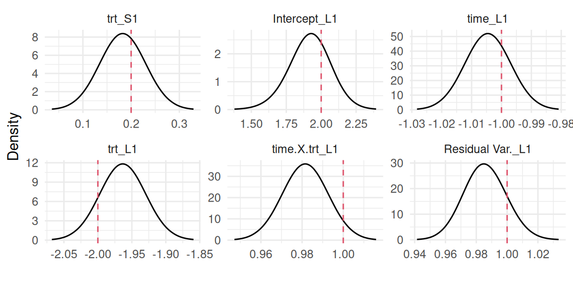
Figure 5.15 shows the baseline hazard of the event:
Plots_jm$Baseline + theme_minimal() + theme(axis.text.y=element_blank(),
                                            axis.ticks.y=element_blank(),
                                            legend.position='none')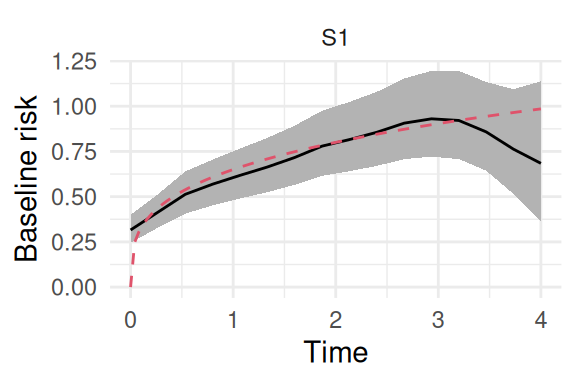
Finally, hyperparameters related to the SPDE includes the standard deviation of the effect, the range of the effect and the scaling of this effect that captures the spatial correlation between longitudinal and survival outcomes:
par(mfrow=c(1,3), mar = c(4,4,2,0.3), cex=0.8)
plot(M_spde$marginals.hyperpar$`Stdev for IDspde_L1`, type="l",
     main="Std. dev.")
plot(M_spde$marginals.hyperpar$`Range for IDspde_L1`, type="l",
     main="Range")
plot(M_spde$marginals.hyperpar$`Beta for SRE_spde_L1_S1`, type="l",
     main="Association")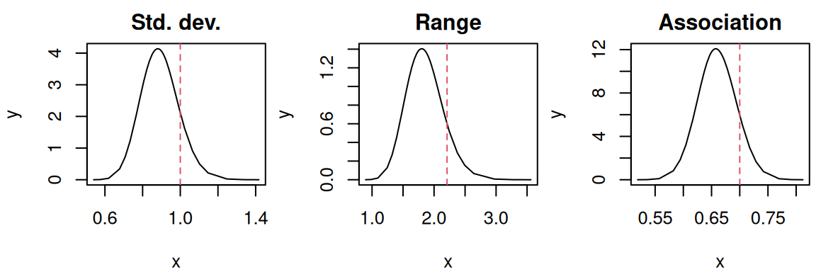
The model did recover the true parameters values. We are also interested in the representation of the spatial random effect over the map. In order to do so, we can evaluate the random effect on a grid of pixels that we can directly plot. First we create a grid with the function fm_evaluator from the package fmesher (Lindgren (2025)):
# grid to project and visualize
grproj <- fm_evaluator(
  mesh = mesh,
  xlim = bb[1, ],
  ylim = bb[2, ],
  dims = round(200 * r2/rr[1])
)
Now we can project the value of the spatial random effect on the grid. In addition to the mean value, we can also project the corresponding standard deviations to get an estimate of the uncertainty over space:
m.grid <- fm_evaluate(grproj, # Mean
  field = M_spde$summary.random$IDspde_L1$mean)
sd.grid <- exp(fm_evaluate(grproj, # Stdev
  field = log(M_spde$summary.random$IDspde_L1$sd)))
We can limit the plot to pixels that fall inside the borders of the map since we projected on a larger rectangle:
gr.in <- st_contains(x = fr1, # which pixels are inside the map
                     y = st_as_sf(as.data.frame(grproj$lattice$loc),
                                  coords = 1:2, crs = st_crs(fr1)))
m.grid[setdiff(1:nrow(grproj$lattice$loc), unlist(gr.in))] <- NA
sd.grid[setdiff(1:nrow(grproj$lattice$loc), unlist(gr.in))] <- NA
Before plotting, we need to convert the data to a raster format, as defined by the terra R package (Hijmans (2025)):
library(terra) # put into raster format
m_raster <- rast(
  data.frame(x = grproj$lattice$loc[, 1], y = grproj$lattice$loc[, 2],
             u = as.vector(m.grid)), crs = "+proj=longlat +datum=WGS84")
sd_raster <- rast(
  data.frame(x = grproj$lattice$loc[, 1], y = grproj$lattice$loc[, 2],
             u = as.vector(sd.grid)), crs = "+proj=longlat +datum=WGS84")
Now we can plot both the mean and standard deviation of the spatial effect, using the R packages ggplot2 (Wickham (2016)) and tidyterra (Hernangómez (2023)):
library(tidyterra)
ggm <- ggplot() + theme_minimal() + geom_spatraster(data=m_raster) +
  scale_fill_distiller(type="div",palette="RdBu",na.value="transparent",
                       label = function(x) sprintf("%.2f", x)) +
  geom_sf(data=fr1,fill='transparent') + ggtitle("Mean effect") +
  theme(axis.title.x=element_blank(), axis.title.y=element_blank())
ggsd <- ggplot() + theme_minimal() + geom_spatraster(data=sd_raster) +
  scale_fill_distiller(type="div",palette="RdBu",
                       na.value="transparent",transf="log",
                       label = function(x) sprintf("%.2f", x)) +
  geom_sf(data=fr1,fill='transparent') + ggtitle("Standard deviation") +
    theme(axis.title.x=element_blank(),axis.title.y=element_blank())
ggarrange(ggm, ggsd)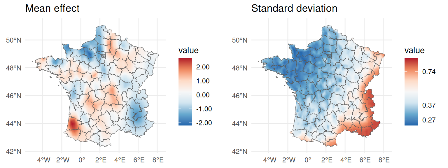
The mean effect captures some variability in space and the standard deviation shows that we have higher uncertainty in the South-East, as expected since we considered less observations in this area compared to North-West where we have many observations and low uncertainty.
It is possible to predict from this model by sampling values from the posterior distribution of the spatial random effect at the desired locations before calling the predict() function. Let’s consider two individuals from the North-West and South-East of the map, as defined by the following coordinates:
pred.loc <- matrix(c(-1.5, 7, 49.5, 44), nrow=2);pred.loc [,1] [,2]
[1,] -1.5 49.5
[2,] 7.0 44.0We can represent these two locations on the map as follows:
ggarrange(ggm + geom_point(aes(x=pred.loc[,1], y=pred.loc[,2]), size=3) +
            theme(legend.position ="none"),
          ggsd + geom_point(aes(x=pred.loc[,1], y=pred.loc[,2]), size=3) +
theme(legend.position = "none")) 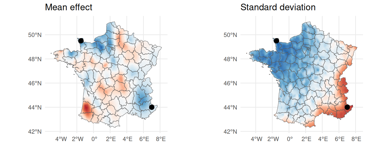
Here we chose locations that are expected to differ both in terms of mean estimate and uncertainty. We define the projector matrix that maps the spatial random effect to the locations of interest by interpolating the surrounding mesh nodes values:
Apred <- apply(pred.loc, 1, function(x)
               fm_evaluator(mesh, matrix(x, nrow = 1))$proj$A)
Now we can sample from the posterior of the full spatial random effect (i.e., we sample values at all the mesh nodes).
NsampleHY <- 20
NsampleFE <- 20
# drawn samples at the mesh nodes
S_samples_mesh <- sapply(inla.posterior.sample(NsampleHY*NsampleFE,M_spde,
  selection=list("IDspde_L1"=1:spde$n.spde)), function(x) x$latent)
Finally, we project the spatial random effect for the new individuals in order to get samples of the posterior distribution of the random effect at their locations. These values are used to quantify the impact and to assess uncertainty related to the spatial random effect in the predictions.
# project the samples for each individual
S_samples_id <- t(sapply(Apred, function(Ai) drop(Ai %*% S_samples_mesh)))
We can now create the dataset for the predictions that includes two lines for our two locations:
ND <- data.frame(id=c("North-West", "South-East"),trt=0,time=0,Y=NA);ND id trt time Y
1 North-West 0 0 NA
2 South-East 0 0 NASince we included the covariate trt in the model, it must be specified to compute predictions, here we assume predictions for both locations conditional on trt=0. The Y is set to NA, so we compute predictions only conditional on the location (i.e., the only difference between our two predictions is the spatial location). It is however possible to also predict conditional on repeated measurements of the marker as presented in Chapter 3 as well as to predict conditional on event times as presented in Chapter 4.
We call the predict function and include the sampled values of the spatial random effect with the argument set.sample:
P <- predict(M_spde, ND, horizon=3, survival=TRUE,
             set.samples=list("IDspde_L1"=S_samples_id))
We can directly plot the predicted longitudinal trajectories as well as the corresponding survival probabilities for these two locations:
ggarrange(ggplot(P$PredL, aes(x=time, y=quant0.5)) +
  geom_ribbon(aes(ymin=quant0.025, ymax=quant0.975), alpha=0.1)+
  geom_line() + theme_minimal() + facet_wrap(~id) + xlab("Time")+
  ylab("Longitudinal marker"),
ggplot(P$PredS, aes(x=time, y=Surv_quant0.5)) + ylim(0,1) +
  geom_ribbon(aes(ymin=Surv_quant0.025, ymax=Surv_quant0.975), alpha=0.1)+
  geom_line() + theme_minimal() + facet_wrap(~id) + xlab("Time") +
ylab("Survival probability"), nrow=2) 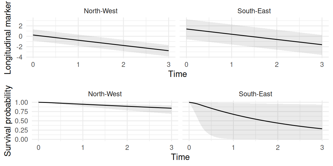
We can clearly see the impact of the uncertainty over the spatial random effect on the predictions of both the longitudinal and survival outcomes.