This chapter explores the analysis of repeatedly measured data using mixed-effects models. We first introduce the linear mixed-effects models followed by generalized linear mixed-effects models, before introducing multivariate outcomes fitted jointly, where correlated random effects capture the relationship between different markers. We also show how INLA can handle more advanced mixed-effects models, including zero-inflated models for counts, two-part models for semicontinuous data and proportional odds models for ordinal data. The chapter finally covers default prior distributions and provides guidance on how to modify them to better fit with specific needs.
Overview of longitudinal models presented in this chapter.
Model
Outcome
Assumption
Section
Linear Mixed Models
Random Intercept
Continuous
Subject-specific baseline heterogeneity.
3.2.3
Random Intercept & Slope
Continuous
Heterogeneity in baseline and rate of change.
3.2.4
Random Effects on Splines
Continuous
Captures non-linear individual trajectories.
3.2.5
Generalized Linear Mixed Models
Poisson Mixed Effects
Count
Model count data using a log link.
3.3.1
Binomial Mixed Effects
Binary/Proportion
Model binary or proportional data using a logit/probit link.
3.3.2
Multivariate & Specialized Models
Multivariate Mixed Model
Multiple
Jointly models multiple longitudinal outcomes via correlated random effects.
3.4
Zero-Inflated Models
Count with excess zeros
A two-component model for the zero-generating and count processes.
3.5
Two-Part Models
Semicontinuous
A two-component model for the zero-generating and continuous processes.
3.6
Tobit Mixed Model
Left-Censored
Models semicontinuous data by treating zeros as censored.
3.7
Proportional Odds Model
Ordinal
Models ordered categorical outcomes.
3.8
3.1 Introduction
Repeated measurements can occur when there is a longitudinal follow-up of patients with repeated visits to measure the same marker. We therefore get multiple values of a marker associated with each individual at different time points. It is common in health research to observe repeated measurements of one or multiple markers of interest. Beyond the direct interest in these markers, they can sometimes capture some important information about the heterogeneity of the data which can be taken into account when analyzing the risk of an event (see Chapter 4).
Longitudinal repeated measurements can have different distributions, where the most commonly observed are:
Continuous values: The measure can take any value.
Semicontinuous values: The measure can take any value in a bounded interval.
Binary values: The measure is either a 0 or a 1.
Counts: The measure is a positive integer.
Proportions or rates The measure can take any value between 0 and 1.
In a longitudinal analysis, each subject \(i\) is designed to be measured at visits \(j\)\((j=1,..., n_i)\), meaning that we expect to collect the full vector of measurements \(Y_i=(Y_{i1}, Y_{i2}, ..., Y_{in_i})^\top\). However, measurement times may be random, and in practice, missing data is common. This missing data can be either intermittent (e.g., a subject misses a visit and returns for the next one) or permanent (e.g., when a subject leaves the study). The mechanisms underlying missing data can be classified into three categories:
Missing completely at random (MCAR): The probability to have a missing data for an individual conditional on the covariates is independent from the observations and missing observations of the marker. Individuals with missing data and individuals with complete records should have the same characteristics under the MCAR assumption. Example: In a clinical trial studying the effect of a treatment on some longitudinal marker measured during blood tests, some participants occasionally miss scheduled measurements due to random events like temporary clinic closures. These missed measurements are unrelated to the participants’ health status or any other variables in the study.
Missing at random (MAR): There are systematic differences between the missing and observed values which can be entirely explained by observed variables. The probability to have a missing data for an individual is therefore related to some other measured covariates in the model, but not to the value of the variable with missing values itself. Example: In a longitudinal study on cognitive decline in elderly adults, participants might skip cognitive assessments if they live far from the clinic. The missingness is related to observed variables (e.g., distance to the clinic) but not directly to their cognitive function.
Missing not at random (MNAR): The probability to have a missing data for an individual is conditional on the covariates as well as the observed and unobserved values of the marker. It is not possible to verify that missing values are MNAR without knowing the missing values. Example: In a study on chronic pain management, participants may drop out because their pain levels have become unbearable, and they seek alternative treatments. The missingness is directly related to the unobserved outcome (severe pain levels) and cannot be explained by other observed variables in the study.
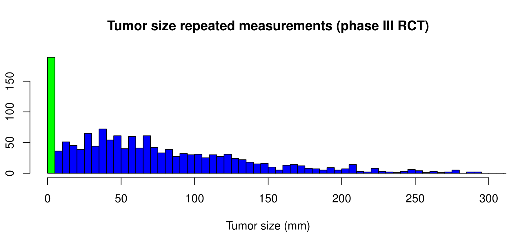
To further illustrate these missing data mechanisms, assume we are interested in the repeated measurements of the tumor size of cancer patients. We have a sample of measurements but some of them are missing. In the situation where the data is MCAR, the probability of a missing measurement is the same for all patients. Now, if older patients have larger tumor sizes and have higher probability of drop-out, the observed sample will not reflect the true distribution of the biomarker from the original population but the distribution of the biomarker conditional on the age of the patients will be similar. The data are therefore MAR because missing values depend on an observed variable (i.e. age). Based on standard missing data theory (Rubin (1976)), likelihood-based methods ignoring the missingness mechanism provide unbiased estimates given that the data are missing at random (MAR) or completely at random (MCAR), because a model can predict the missing data to obtain unbiased estimates (Verbeke & Molenberghs (2000)). Finally, if patients with higher tumors size are less likely to produce measurements (e.g., because of the disability provoked by the large tumors themselves), the distribution of the observed tumors will differ from the distribution in the population of interest. When the missingness mechanism depends on some unobserved aspect of the data, i.e., the data are missing not at random (MNAR), regression methods may be biased for certain parameters (Fitzmaurice et al. (1995), Molenberghs & Verbeke (2001), Kurland & Heagerty (2005), Rouanet et al. (2019)). It is a fundamentally untestable assumption, because it concerns the unobserved values. Therefore, the assumption needs to be justified based on background knowledge and discussion with experts. In case missing data are the result of informative drop-out (e.g. death), the marker measurements and the drop-out mechanism have to be jointly modeled to obtain valid estimates (see Chapter 4).
In longitudinal data analysis, we are interested in the effect of covariates on the values of the longitudinal marker. Through regression models, we can evaluate how the baseline values of the marker as well as the evolution over time compares conditional on given covariates. The simple linear regression model captures the population average effect of covariates on the distribution of the marker, but our focus here is on the individual level (or any grouping level), where we aim to account for each subject’s deviation from this average effect. This is possible because repeated measurements of the marker informs about individual-specific characteristics.
The longitudinal models presented in this chapter capture temporal evolution through linear trends or more flexible spline-based functions. While these approaches are powerful, they are not the only options for modeling the correlation structure inherent in repeated measurements over time. Other methods not presented in this chapter are available within the INLA framework to handle such dependencies (e.g., AR1).
3.2 Linear mixed-effects models
3.2.1 Description
The linear mixed-effects (LME) model (Harville (1977), Laird & Ware (1982)) is an extension of the simple linear regression model that allows the inclusion of both fixed and random effects to model a continuous marker. Fixed effects corresponds to the effect of observed variables, it is constant across individuals while a random effect corresponds to group-specific effect of latent (i.e., unobserved) variables. The inclusion of random effects in a fixed effects model assists in controlling the unobserved heterogeneity. LME models are particularly useful for data with a hierarchical structure, for which the independence assumption is violated. The structure of the data can be decomposed into groups that share some common variability in the measurements. In the context of individual repeated measurements, each individual is a group and there is a variability intra-groups (i.e., between repeated measurements of the same individual) and a variability inter-groups (i.e., between individuals).
Let \(Y_{ij}\) denote the biomarker measurement of subject \(i\) (\(i=1,...,n\)) at time \(j\) (\(j=1,...,n_i\)) and \(Y_i=(Y_{i1},Y_{i2},...,Y_{in_i})^\top\) the vector of responses for subject \(i\). We assume the observed biomarker value is noisy (e.g., due to the precision of the tools used to produce the measure), the true value of the biomarker \(Y^*\) remains unobserved and the following linear mixed-effect model for individual \(i\) at any time \(t>0\) is supposed,
\[\begin{align*}
Y_{i}(t)=Y_{i}(t)^*+\epsilon=X_{i}(t)^\top \beta+Z_{i}(t)^\top b + \epsilon.\\
\end{align*}\]
The explanatory variables \(X\) and \(Z\) are associated with the fixed effects regression coefficients \(\beta\) and the random effects \(b\), respectively. The random effects are assumed to be Gaussian distributed and possibly correlated \(b|\Sigma_b \sim \mathcal{N}(0, \Sigma_b)\). The measurement error \(\epsilon\) follows a Gaussian distribution \(\mathcal{N}(0, \sigma_{\epsilon}^2)\) and is assumed independent from the random effects. The repeated measures of \(Y\) are assumed independent conditional on the fixed and random effects. Random effects account for unobserved confounders that affect the individual, such as genetic or environmental exposure. Sometimes, additional levels of hierarchy can explain some variability shared between individuals (e.g., geographical areas or shared genetic features). The model gives the marginal expectation of \(Y_{i}(t)\) for the entire population sharing features \(X\) through the term \(X^\top \beta\) and the subject-specific expectation of \(Y_{ij}\) by \(X_{ij}^\top\beta+Z_{ij}^\top b\). The corresponding likelihood function is \[\begin{align*}
L(\Theta)&=\prod_{i=1}^{n} \prod_{j=1}^{n_i} p(Y_{ij}),\\
&= \prod_{i=1}^{n} \prod_{j=1}^{n_i} \int_{b} p_N(Y_{ij}|b)p(b)\mathrm{d}b,
\end{align*}\] where \(p_N\) is the Gaussian density evaluated at \(Y_{ij}\) (other densities are discussed in Section 3.3).
As shown in Chapter 1, if we assume a Gaussian prior for \(\varphi = \{\beta, b\}\), then due to the conditional independence of the data \(Y\), the linear mixed-effects model is an LGM and we can thus use INLA to perform approximate Bayesian inference of this model.
3.2.2 Fixed effects only model
We first introduce a simple linear regression model, defined as follows: \[\textrm{E}[Y_{i}(t)]=\beta_0 + \beta_1\cdot t + \beta_2\cdot trt_i + \beta_3\cdot trt_i\cdot t \] where:
\(Y_{i}(t)\) is the outcome for individual \(i\) at time \(t\).
\(\beta_0\) is the population intercept, representing the mean outcome at \(t\)=0 for the reference group (here, \(trt\)=0).
\(\beta_1\) is the population slope, representing the rate of change in the outcome over time for the reference group.
\(\beta_2\) is the effect of the treatment on the intercept (i.e., at \(t\)=0).
\(\beta_3\) is the interaction effect, representing the difference in the slope between the treatment and reference groups.
In order to simulate from this model, we simply compute the value of the linear combination of the fixed effects for different individuals at different time points. Then, we add random Gaussian noise with variance \(\sigma_\epsilon^2 = 1\).
n=50# number of individualsb_0=2# interceptb_1=-1# slopeb_2=-2# trtb_3=1# trt x slopeb_e=1# residual errormestime=seq(0, 5, 1) # measurement timesn_i <-length(mestime)time=rep(mestime, n) # time columnid<-rep(1:n, each=n_i) # individual idtrt=rep(rbinom(n, 1, 0.5), each=n_i) # binary trt covariatelinPred <- b_0 + b_1*time + b_2*trt + b_3*trt*time # linear predictorY <-rnorm(n_i*n, linPred, b_e) # observed outcomedatL <-data.frame(id, time, Y, trt=as.factor(trt))summary(datL) # longitudinal dataset
       id            time           Y            trt
 Min.   : 1.0   Min.   :0.0   Min.   :-5.28524   0:138
 1st Qu.:13.0   1st Qu.:1.0   1st Qu.:-1.12259   1:162
 Median :25.5   Median :2.5   Median :-0.09918
 Mean   :25.5   Mean   :2.5   Mean   :-0.18900
 3rd Qu.:38.0   3rd Qu.:4.0   3rd Qu.: 0.78008
 Max.   :50.0   Max.   :5.0   Max.   : 4.49766
We can have a look at the simulated individual trajectories:
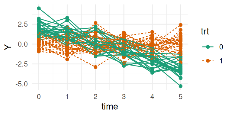
library(ggplot2)ggplot(datL, aes(time, Y, group = id, color = trt, linetype = trt)) +geom_point() +geom_line() +theme_minimal()
Figure 3.1: Simulated individual longitudinal trajectories from a linear model without random effects. Each line represents an individual’s data over time, with colors and line type distinguishing between the two treatment groups. Trajectories are parallel, with variation arising only from fixed effects and residual error.
Here we can see how the two treatment lines have a different intercept and a different slope. Note that here the only difference between individuals that share the same treatment line is coming from the residual Gaussian error term. For simplicity, we assume the same visit times and no intermittent missing values, although these are often observed in real data, it is not expected to affect the results under the MCAR assumption.
We can fit this model with R-INLA as follows:
library(INLA)M_LinReg <-inla(formula = Y ~ time*trt, data=datL)summary(M_LinReg)
Time used:
    Pre = 0.549, Running = 0.164, Post = 0.0145, Total = 0.728
Fixed effects:
              mean    sd 0.025quant 0.5quant 0.975quant   mode kld
(Intercept)  2.179 0.147      1.892    2.179      2.467  2.179   0
time        -1.036 0.048     -1.131   -1.036     -0.941 -1.036   0
trt1        -2.118 0.199     -2.510   -2.118     -1.727 -2.118   0
time:trt1    1.012 0.066      0.882    1.012      1.141  1.012   0

Model hyperparameters:
                                        mean    sd 0.025quant 0.5quant 0.975quant mode
Precision for the Gaussian observations 1.07 0.087      0.902     1.06       1.24 1.06

Marginal log-Likelihood:  -447.19
 is computed
Posterior summaries for the linear predictor and the fitted values are computed
(Posterior marginals needs also 'control.compute=list(return.marginals.predictor=TRUE)')
The summary of the results include the fixed effects first, followed by the hyperparameters which here consists of the residual error precision (i.e., inverse of variance). While the precision is mathematically convenient, variance or standard deviation is often more intuitive. The posterior mean of the residual variance can be calculated as \(\sigma_\epsilon^2=1/\) 1.07 \(\simeq\) 0.94. This value quantifies the variance of the deviation of observed data points from the mean regression line defined by the fixed effects. The true value used in the simulation was \(\sigma_\epsilon^2=1\), so the model has successfully recovered this parameter given the 95% credible interval.
The marginal log-likelihood is also provided, which can be useful for model comparison but some goodness of fit metrics are also available with INLA, as illustrated later in this chapter.
The marginal posterior densities of the fixed effects are directly available in the marginals.fixed argument:
str(M_LinReg$marginals.fixed)
List of 4
 $ (Intercept): num [1:43, 1:2] 1.55 1.63 1.72 1.84 1.89 ...
  ..- attr(*, "dimnames")=List of 2
  .. ..$ : NULL
  .. ..$ : chr [1:2] "x" "y"
 $ time       : num [1:43, 1:2] -1.24 -1.22 -1.19 -1.15 -1.13 ...
  ..- attr(*, "dimnames")=List of 2
  .. ..$ : NULL
  .. ..$ : chr [1:2] "x" "y"
 $ trt1       : num [1:43, 1:2] -2.98 -2.87 -2.74 -2.58 -2.51 ...
  ..- attr(*, "dimnames")=List of 2
  .. ..$ : NULL
  .. ..$ : chr [1:2] "x" "y"
 $ time:trt1  : num [1:43, 1:2] 0.727 0.764 0.807 0.858 0.882 ...
  ..- attr(*, "dimnames")=List of 2
  .. ..$ : NULL
  .. ..$ : chr [1:2] "x" "y"
We can plot the posterior marginals of the fixed effects and compare to the true values used to generate the data:
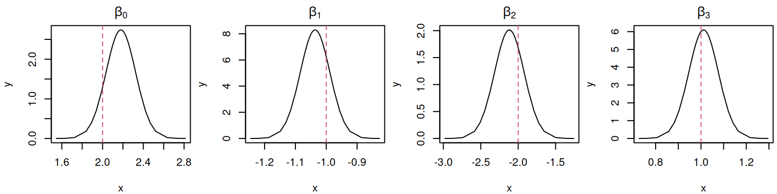
par(mfrow=c(1,4), mar =c(4,4,2,0.3))plotF <-function(x) {plot(M_LinReg$marginals.fixed[[x]], type="l",main=eval(parse(text=(paste0("expression(beta[", x-1, "])")))))}sapply(1:4, plotF)
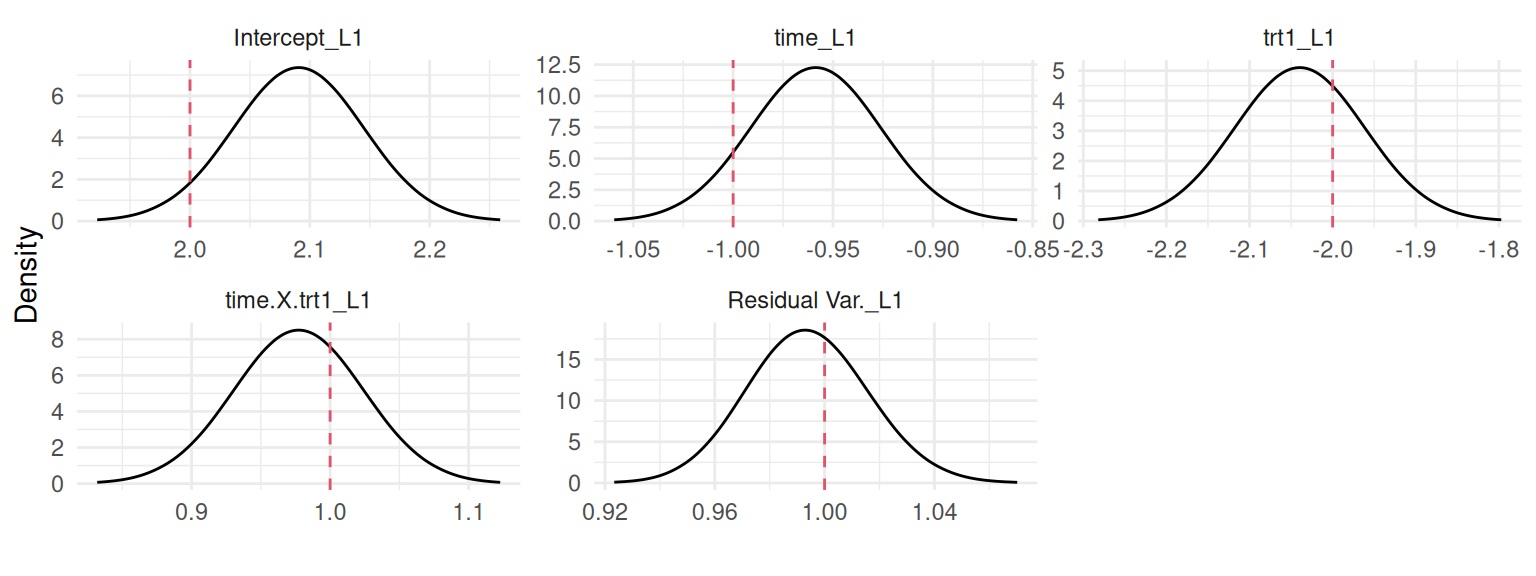
Figure 3.2: Posterior marginal distributions of the fixed effects from a simple linear regression model for the intercept (\(\beta_0\)), time (\(\beta_1\)), treatment (\(\beta_2\)), and the interaction (\(\beta_3\)). Dashed red lines indicate the true values used for data generation.
The remaining parameter is the residual error, which is presented through its precision in the R-INLA summary. Since it is a hyperparameter, its marginal posterior density is available in the argument marginals.hyperpar of the fitted object:
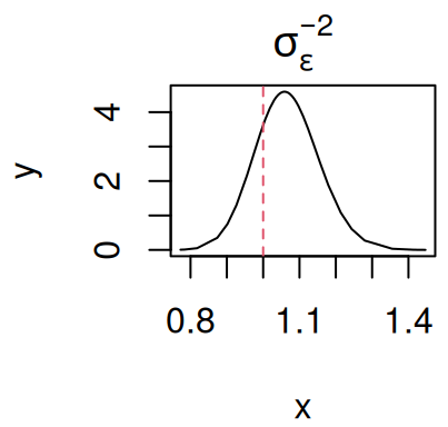
par(mfrow=c(1,1), mar =c(4,4,2,0.3))plot(M_LinReg$marginals.hyperpar[[1]],type="l", main=expression(sigma[epsilon]^-2))
Figure 3.3: Posterior marginal distribution of the residual error precision (\(\sigma_{\epsilon}^{-2}\)). The dashed red line indicates the true value.
Note that it is possible to transform posterior marginals by applying any function and therefore we could get the posterior density of the variance of the residual error, by applying the inverse function. This is done with the inla.tmarginal() function and an example of the use of this function is presented in Section 2.2.1.
3.2.3 Random intercept model
Let’s consider the previous model but we now include a random intercept, such that each individual has a specific deviation from the average value at baseline. The model is then defined as follows \[\textrm{E}[Y_{i}(t)]=\beta_0 + b_i + \beta_1\cdot t + \beta_2\cdot trt_i + \beta_3\cdot trt_i\cdot t \] where \(b_i\) is the random intercept for individual \(i\) with a Gaussian distribution \(\mathcal{N}(0, \sigma_b^2)\) which captures the unobserved, time-invariant heterogeneity between individuals. The simulation scheme follows trivially from the previous model, where we first generate the random intercept values, compute the linear combination of fixed and random effects and add noise (i.e. residual error). The observed data has a hierarchical structure where observations within the same individual are correlated because they share the same random intercept \(b_i\).
n=1000# number of individualsb_intSD=1# random intercept standard deviationtime=rep(mestime, n) # time columnid<-rep(1:n, each=n_i) # individual idb_int <-rep(rnorm(n, mean=0, sd=b_intSD), each=n_i) # random intercepttrt=rep(rbinom(n, 1, 0.5), each=n_i) # binary trt covariatelinPred <- b_0 + b_int + b_1*time + b_2*trt + b_3*trt*time # predictorY <-rnorm(n_i*n, linPred, b_e) # observed outcomedatLME <-data.frame(id, time, Y, trt=as.factor(trt))summary(datLME) # longitudinal dataset
       id              time           Y           trt
 Min.   :   1.0   Min.   :0.0   Min.   :-7.3528   0:3114
 1st Qu.: 250.8   1st Qu.:1.0   1st Qu.:-1.5016   1:2886
 Median : 500.5   Median :2.5   Median :-0.2022
 Mean   : 500.5   Mean   :2.5   Mean   :-0.2776
 3rd Qu.: 750.2   3rd Qu.:4.0   3rd Qu.: 1.0086
 Max.   :1000.0   Max.   :5.0   Max.   : 6.5767
and we can plot the individual trajectories:
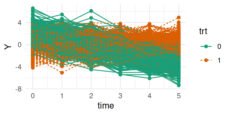
library(ggplot2)ggplot(datLME, aes(time, Y, group = id, color = trt, linetype = trt)) +geom_point() +geom_line() +theme_minimal()
Figure 3.4: Simulated individual longitudinal trajectories from a random intercept model. Subject-specific random intercepts result in parallel trajectories with unique vertical shifts for each individual.
Despite the increased number of individuals, the trajectories in Figure 3.4 look similar to the first model, although here there is a variability between individual coming from the random intercept in addition to the residual variability between all observations captured by the residual error term.
In order to fit this model with R-INLA, we need to introduce the f() terms which are used to define any random effects. In our case, we are interested in a single independent and identically distributed (i.e., iid) random effect. Of note, this is presented for transparency and clarity in how R-INLA deals with random effects but INLAjoint facilitates this process by using a more common R syntax similar to lme4 R package (Bates et al. (2015)).
Time used:
    Pre = 0.275, Running = 0.338, Post = 0.0632, Total = 0.676
Fixed effects:
              mean    sd 0.025quant 0.5quant 0.975quant   mode kld
(Intercept)  1.930 0.056      1.821    1.930      2.039  1.930   0
time        -0.987 0.011     -1.008   -0.987     -0.967 -0.987   0
trt1        -1.924 0.080     -2.081   -1.924     -1.767 -1.924   0
time:trt1    0.987 0.015      0.957    0.987      1.017  0.987   0

Random effects:
  Name    Model
    id IID model

Model hyperparameters:
                                         mean    sd 0.025quant 0.5quant 0.975quant  mode
Precision for the Gaussian observations 0.981 0.020      0.943    0.980       1.02 0.980
Precision for id                        0.939 0.049      0.846    0.937       1.04 0.935

Marginal log-Likelihood:  -9614.20
 is computed
Posterior summaries for the linear predictor and the fitted values are computed
(Posterior marginals needs also 'control.compute=list(return.marginals.predictor=TRUE)')
Similar as the residual error term, the random effect is defined by its precision, with marginal posteriors directly available in the fitted object in the argument marginals.hyperpar:
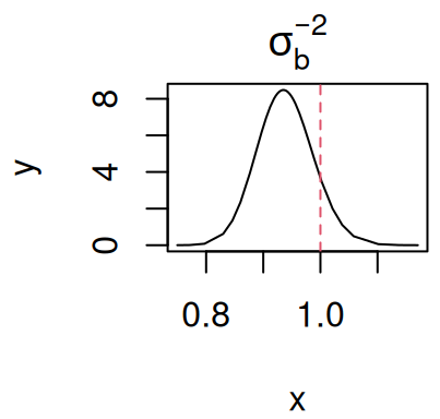
par(mfrow=c(1,1), mar =c(4,4,2,0.3))plot(M_LME_inla$marginals.hyperpar$`Precision for id`, type="l",main=expression(sigma[b]^-2))
Figure 3.5: Posterior marginal distribution of the random intercept precision (\(\sigma_{b}^{-2}\)). The dashed red line indicates the true value.
Beyond the precision of the random effect, R-INLA also gives the posterior distribution of each group-specific random effect (here, for each individual), with a summary available in the summary.random argument of the fitted object while marginals are available in marginals.random. For example the marginal posterior estimates of the random intercept for the first two individuals in the simulated dataset are:
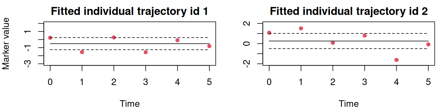
We can check how these values fit with the observed data by comparing them with the estimated linear predictor for these first two individuals. The linear predictor for each data observation included for the model fit is available in the summary.linear.predictor argument (while the corresponding marginals are in marginals.linear.predictor):
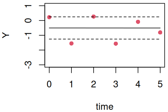
Figure 3.6: Fitted individual trajectories for the first two subjects from a random intercept model. Points are observed data. The solid line is the posterior mean of the fitted linear predictor, and dashed lines form the 95% credible interval.
Of course here the model is very simple, but INLA can become cumbersome for fitting longitudinal models, especially when dealing with multiple random effects as demonstrated in the following subsection. Additionally, INLA presents results in a format that may not align with our primary interests, such as focusing on the precision of random effects or residual errors rather than variances or standard deviations. We will now illustrate how to use INLAjoint to fit these models, highlighting its user-friendly interface, which is particularly advantageous for more complex models. The random intercept regression model can be inferred using INLAjoint as follows:
library(INLAjoint)M_lme <-joint(formLong = Y ~ time * trt + (1|id),dataLong=datLME, id ="id", timeVar ="time")
The formLong argument corresponds to the formula for the mixed-effects model. The structure of the formula is similar to the commonly used structure from the R package lme4 (Bates et al. (2015)), which includes random effects as (NAME | ID), where NAME is the column that contains the variable to weight the random effects (1 corresponding to random intercept) and ID is the name of the grouping variable (e.g., individual id). The dataLong argument is the dataset that must contain the variables given in formLong. Argument id is the name of the column to identify repeated measurements (e.g., individuals) while the timeVar argument gives the name of the time variable column. We can check the summary of this model:
The summary is structured differently as the raw R-INLA output, it first displays the fixed effects and residual error variance and then the variance-covariance of the random effects. As for survival models presented in the previous chapter, the log marginal-likelihood, the Deviance Information Criterion (DIC, Spiegelhalter et al. (2002)) and the Widely Applicable Bayesian Information Criterion (WAIC, Watanabe (2013)) are directly provided in the model summary. It is possible to switch from variance terms to standard deviations by adding the argument sdcor=TRUE in the call of the summary function:
Now the residual error term and the random intercept are described by their posterior standard deviations.
The value \(\sigma_b=\) 1.03 is the posterior mean of the standard deviation of the random intercept. It measures the amount by which an individual’s baseline intercept deviates from the population average intercept (i.e., \(\beta_0\)). Since the random intercepts are assumed to be normally distributed, we can state that approximately 95% of individuals have a true baseline intercept (\(\beta_0 + b_i\)) that falls within the range of \(\beta_0 \pm 1.96 \cdot \sigma_b\) which gives approximately the interval [-0.1, 3.95].
The plot function applied to a longitudinal model fitted with INLAjoint returns a series of plots, starting with the posterior marginal densities shown in Figure 3.7:
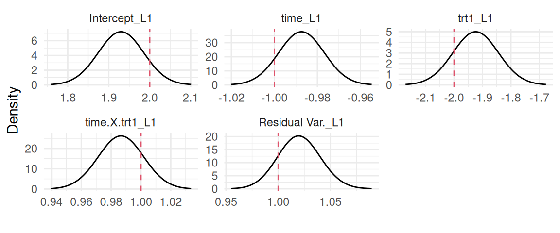
plot(M_lme)$Outcomes$L1
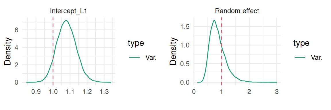
Figure 3.7: Posterior marginal densities of the fixed effects and residual variance from a random intercept model. Dashed red lines indicate the true values used for data generation.
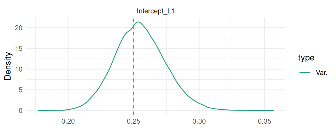
The second plot is the variance of the random intercept:
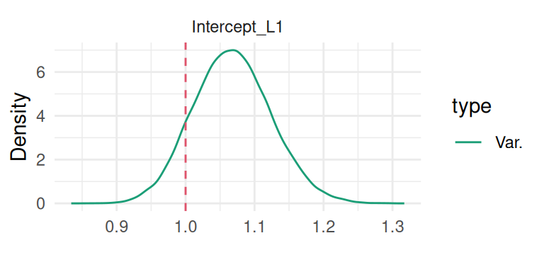
plot(M_lme)$Covariances$L1
Figure 3.8: Posterior marginal distribution of the random intercept variance. The dashed red line indicates the true value.
Since INLAjoint is an interface that facilitates the use of INLA, it returns objects with the same structure as models fitted directly with R-INLA. Therefore, we can see the posterior summary of the random effects in the summary.random argument of the fitted object while the marginal posterior densities are in the marginals.random argument.
  ID       mean        sd 0.025quant   0.5quant 0.975quant
1  1 -0.5100495 0.3854531  -1.265909 -0.5100488  0.2458066
2  2  0.2512217 0.3854396  -0.504609  0.2512213  1.0070541
Here we can see the same posterior distribution for the random intercept as found earlier with the R-INLA fit. Similarly, the linear predictor for each fitted value of the outcome is available in the argument summary.linear.predictor:
Figure 3.9: Fitted individual trajectory for the first individual from a random intercept model. The points are observed data, and the solid line is the posterior mean of the fitted linear predictor with its 95% credible interval (dashed lines).
Here the underlying trajectory is given by the model. Note that this trajectory includes a 95% credible interval to quantify uncertainty around the true underlying value of the outcome (i.e., the residual error from observed marker values is excluded). A 95% credible interval over the observed values would require to also include the residual error source of variability (see Section 3.2.5).
3.2.4 Random intercept and slope model
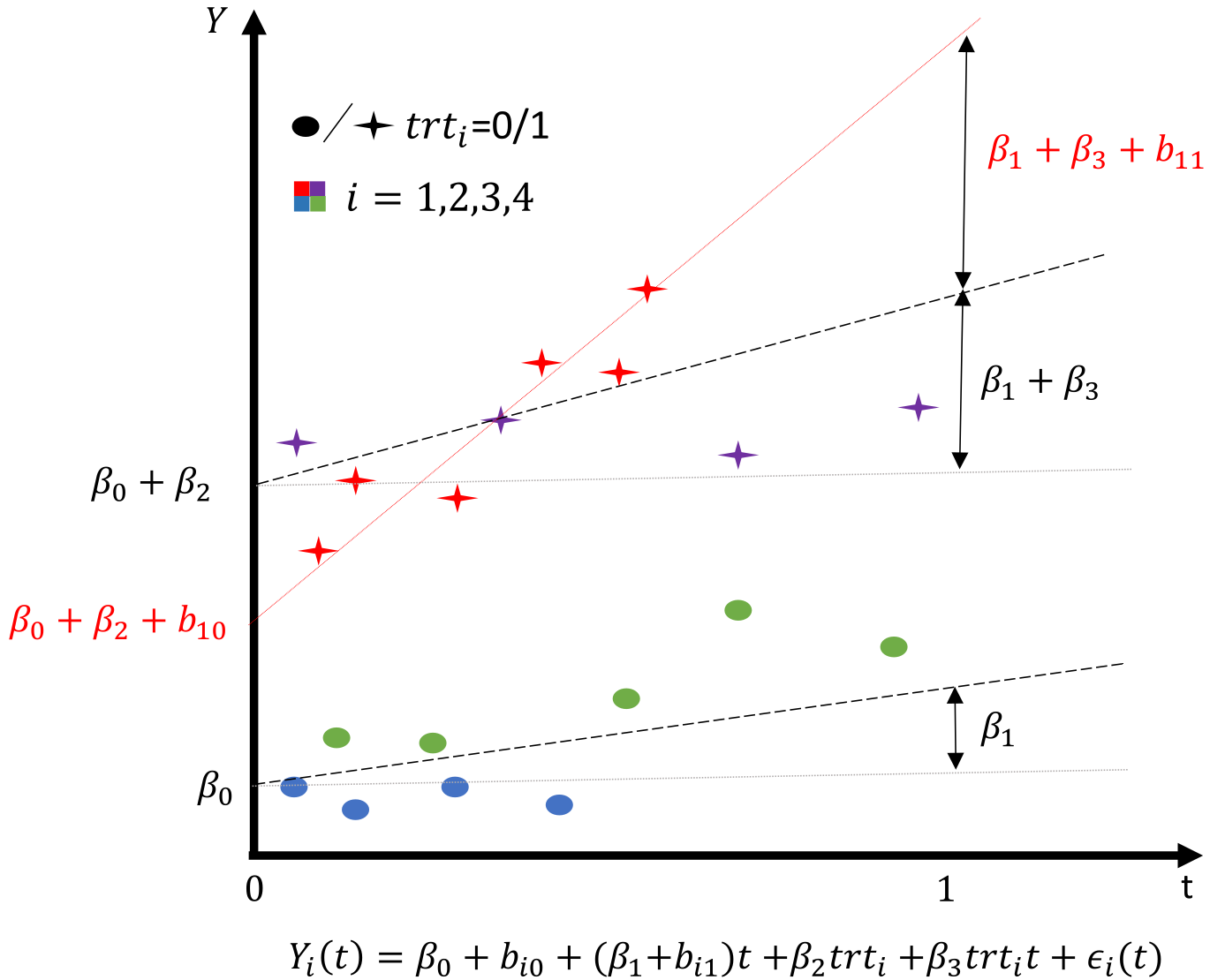
We have seen how to incorporate a random intercept in a mixed-effects model for a longitudinal outcome. Let’s now increase flexibility by including a random slope and considering the correlation between the random intercept and slope, allowing each individual to have their own baseline value and evolution over time. The correlation parameter will inform about the relationship between deviation from average at the intercept and over the slope, such that an individual with a higher/lower value at baseline may be associated to a steeper/lighter evolution over time. We consider the following model: \[\textrm{E}[Y_{i}(t)]=\beta_0 + b_{i0} + (\beta_1 + b_{i1})\cdot t + \beta_2\cdot trt_i + \beta_3\cdot trt_i\cdot t \] where \(b_i\) is a vector of random effects that includes a random intercept \(b_{i0}\) and a random slope \(b_{i1}\). They follow a multivariate Gaussian distribution \(N(0, \Sigma_b)\), with \(\Sigma_b = \begin{pmatrix} \sigma_{b_0}^2 & \sigma_{b_{01}}\\ \sigma_{b_{01}} & \sigma_{b_1}^2\end{pmatrix}\). The parameter \(\sigma_{01}\) captures the covariance between the random intercept and the random slope.
In order to better understand the role of each parameter in the model, the following illustration shows how the fixed and random effects describe population average and individual trajectories over 4 individuals:
Illustration of a linear mixed-effects model with random intercept and slope.
The colors corresponds to the different individuals and the type of point corresponds to a binary covariate such as treatment. Population average estimates are shifted by random effects to fit individual trajectories.
The simulation strategy differs from the previous model as we now need to sample correlated random effects from a bivariate distribution. This is done with the rmvnorm() function from the R package mvtnorm (Genz & Bretz (2009)).
library(mvtnorm) # to sample from multivariate Gaussianb_sloSD=0.7# random slope standard deviationcor_bintslo=0.6# correlationcov_bintslo <- b_intSD*b_sloSD*cor_bintslo # covarianceSigma=matrix(c(b_intSD^2, cov_bintslo, # variance-covariance matrix cov_bintslo, b_sloSD^2), ncol=2)MVnorm <-rmvnorm(n, rep(0, 2), Sigma) # sample from multivariate normalb_int <-rep(MVnorm[,1], each=n_i) # random interceptsb_slo <-rep(MVnorm[,2], each=n_i) # random slopeslinPred <- b_0 + b_int + (b_1 + b_slo)*time + b_2*trt + b_3*trt*timeY <-rnorm(n_i*n, linPred, b_e) # observed outcomedatLME2 <-data.frame(id, time, Y, trt=as.factor(trt))summary(datLME2) # longitudinal dataset
       id              time           Y            trt
 Min.   :   1.0   Min.   :0.0   Min.   :-18.7201   0:3114
 1st Qu.: 250.8   1st Qu.:1.0   1st Qu.: -1.8383   1:2886
 Median : 500.5   Median :2.5   Median :  0.1615
 Mean   : 500.5   Mean   :2.5   Mean   : -0.1117
 3rd Qu.: 750.2   3rd Qu.:4.0   3rd Qu.:  1.9496
 Max.   :1000.0   Max.   :5.0   Max.   : 14.3885
ggplot(datLME2, aes(time, Y, group = id, color = trt, linetype = trt)) +geom_point() +geom_line() +theme_minimal()
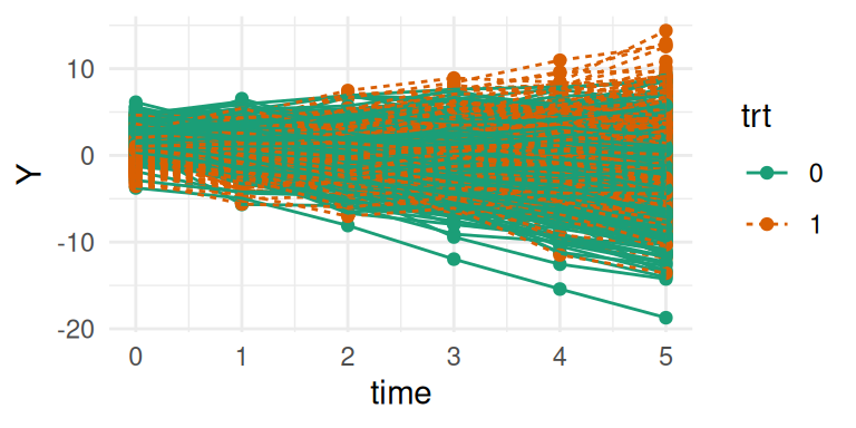
Figure 3.10: Simulated individual longitudinal trajectories from a random intercept and slope model.
We start by showing how to fit the model with R-INLA for educational purpose but it is easier to fit this model (and more complex models) with INLAjoint which will be used for the rest of the chapter. Since we already introduced the random effects with R-INLA for the random intercept model, we can add the random slope in a similar way. It is however important to have unique columns for each random effect, we therefore first need to duplicate the column id to setup the id for the slope (ids):
datLME2$ids <- datLME2$idM_LME2_inla <-inla(formula = Y ~ time*trt +f(id, model="iid") +f(ids, time, model="iid"), data=datLME2)summary(M_LME2_inla)
Time used:
    Pre = 0.294, Running = 0.463, Post = 0.0937, Total = 0.851
Fixed effects:
              mean    sd 0.025quant 0.5quant 0.975quant   mode kld
(Intercept)  2.091 0.058      1.977    2.091      2.204  2.091   0
time        -0.959 0.035     -1.027   -0.959     -0.891 -0.959   0
trt1        -2.040 0.083     -2.203   -2.040     -1.876 -2.040   0
time:trt1    0.977 0.050      0.879    0.977      1.075  0.977   0

Random effects:
  Name    Model
    id IID model
   ids IID model

Model hyperparameters:
                                         mean    sd 0.025quant 0.5quant 0.975quant  mode
Precision for the Gaussian observations 1.035 0.023      0.991    1.034      1.080 1.034
Precision for id                        0.816 0.051      0.720    0.815      0.922 0.811
Precision for ids                       1.767 0.086      1.604    1.765      1.942 1.762

Marginal log-Likelihood:  -10860.08
 is computed
Posterior summaries for the linear predictor and the fitted values are computed
(Posterior marginals needs also 'control.compute=list(return.marginals.predictor=TRUE)')
The random slope is weighted with time, which is included as the second argument of the f() call. Now we have our two random effects but they are independent. In order to have correlated random effects, we can use the multivariate iid model named iidkd. It requires giving the order k and the size n which is here two times the number of individuals for the two random effects. Correlated random effects require unique id for each random effect and each individual, such that our random slope must start with the id max(id)+1 and end with max(id)*2, we can create a new column for this id:
datLME2$ids2 <- datLME2$id +max(datLME2$id)
Now we can fit the model with two correlated random effects, where the first f() call does setup the bivariate random effect with the random intercept id (id) and the second f() call has the copy argument to setup the random slope id (ids2):
M_LME2_inla <-inla(formula = Y ~ time*trt +f(id, model="iidkd", order=2, n=2*n) +f(ids2, time, copy="id"), data=datLME2)summary(M_LME2_inla)
Time used:
    Pre = 0.537, Running = 0.801, Post = 0.157, Total = 1.49
Fixed effects:
              mean    sd 0.025quant 0.5quant 0.975quant   mode kld
(Intercept)  2.091 0.053      1.986    2.091      2.196  2.091   0
time        -0.959 0.032     -1.022   -0.959     -0.895 -0.959   0
trt1        -2.040 0.077     -2.191   -2.040     -1.889 -2.040   0
time:trt1    0.977 0.047      0.886    0.977      1.069  0.977   0

Random effects:
  Name    Model
    id IIDKD model
   ids2 Copy

Model hyperparameters:
                                          mean    sd 0.025quant 0.5quant 0.975quant   mode
Precision for the Gaussian observations  0.999 0.023      0.955    0.999      1.044  0.998
Theta1 for id                            0.263 0.056      0.154    0.262      0.375  0.259
Theta2 for id                            0.363 0.025      0.315    0.363      0.412  0.363
Theta3 for id                           -1.131 0.115     -1.362   -1.129     -0.911 -1.121

Marginal log-Likelihood:  -10803.62
 is computed
Posterior summaries for the linear predictor and the fitted values are computed
(Posterior marginals needs also 'control.compute=list(return.marginals.predictor=TRUE)')
The random effects are parameterized with the Cholesky of the precision matrix (i.e., inverse of covariance) in INLA, therefore the results here (“Theta for id”) cannot be directly interpreted. This parametrization replaces the previous INLA default for multivariate random effects which was using the precision and correlation internally. This new parametrization allows for more numerical stability and can better scale for higher dimensions. We can sample from the posterior distribution of the theta parameters (with the function inla.iidkd.sample()) and convert to the desired scale, i.e., covariance or standard deviations and correlations (the argument return.cov allows to choose between variance and standard deviation). We can have a look at the variance-covariance parameters and compare to true values:
We can see that the model is able to find true values for the variance and covariance of the random effects.
With INLAjoint, the additional random slope can simply be included in the random effects part of the formula, such that (1 + time|id) indicates the inclusion of correlated random intercept and slope:
M_lme2 <-joint(formLong = Y ~ time * trt + (1+ time|id),id ="id", timeVar ="time", dataLong=datLME2)summary(M_lme2)
We now have 3 parameters related to individual random effects. While the interpretation of variances is similar to the random intercept model, the covariance provides a new information about the data. A positive covariance indicates that individuals who start with a higher than average baseline value (i.e., positive \(b_{i0}\)) also tend to have a steeper than average slope (i.e., positive \(b_{i1}\)). While the covariance indicates the direction of the relationship, the correlation is a more interpretable, scale-free measure of its strength. By calling summary(M_lme2, sdcor=TRUE), we obtain the standard deviations and the correlation directly.
A correlation of 0.59 suggests a moderately strong positive association between individuals’ baseline values and their rates of change. In a clinical context, this could mean that patients with a more severe initial condition (higher value at baseline) also experience a more rapid change (e.g., faster decline or faster response to treatment) over the course of the study.
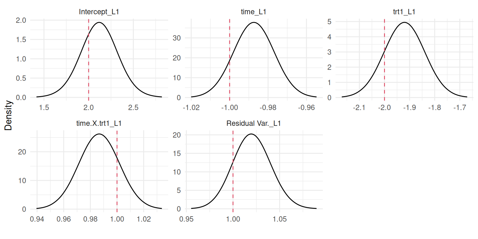
We can see that our model properly captures all the fixed effects by displaying their posterior marginals with the plot() function:
plot(M_lme2)$Outcomes$L1
Figure 3.11: Posterior marginal distributions of the fixed effects and residual standard deviation from a random intercept and slope model. Dashed red lines indicate the true values.
And similarly we can display the variance-covariance of the two correlated random effects:
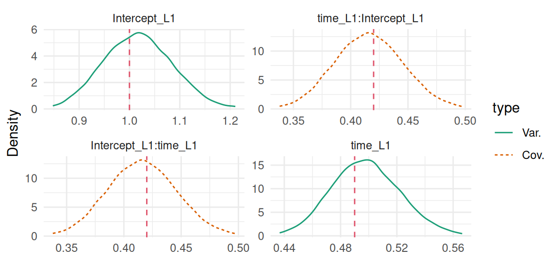
plot(M_lme2)$Covariances$L1
Figure 3.12: Posterior marginal distributions of the variance-covariance components for the random effects: variance of the random intercept, variance of the random slope and their covariance. Dashed vertical red lines indicate the true values.
We can have a look at the fitted trajectory for the first individual:
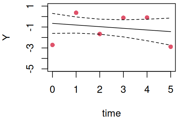
Figure 3.13: Fitted individual trajectory for a subject from a random intercept and slope model. Points are observed data. The solid line is the posterior mean of the fitted linear predictor, with dashed lines for the 95% credible interval.
We can see how the model is able to capture increasing/decreasing trends but still remains very simple as it assume linear trajectories.
Note that the vector of random effects for a given longitudinal submodel with default INLAjoint options have an unspecified covariance structure (i.e., full correlation between all random effects) but can be switched to independent random effects with the boolean argument corRE:
M_lme2 <-joint(formLong = Y ~ time * trt + (1+ time|id),id ="id", timeVar ="time", corRE=FALSE,dataLong=datLME2)summary(M_lme2, sdcor=T)
Here we can see that we did not consider the correlation between the random intercept and slope.
3.2.5 Random intercept and splines model
In order to have more flexibility for the trajectory of the marker over time, we can include functions of time. With INLAjoint, functions of time can be included in formulas, they first need to be set up as a univariate function with name fX, where X is a number starting with 1 and incrementing for each additional function of time required. Then the function can be used directly in the formula of a longitudinal model. While it is possible to apply the function of time before calling the joint() function, it is important to provide the function for multiple reasons. First, the computation of predictions requires to know this function, otherwise the functions of time are interpreted as stepwise constant. Moreover in the context of joint modeling where the linear predictor of the longitudinal models, including functions of time, can be shared in a survival submodel, the shared part needs to be computed at many time points internally to properly account for its evolution over time in the risk function (see Section 4.3.2).
Let’s consider a model that includes two cubic splines basis for the fixed and random effects of time, with an interaction with a binary covariate trt. The model is defined as follows: \[\begin{align*}
\textrm{E}[Y_{i}(t)]=&\beta_0 + b_{i0} + (\beta_1 + b_{i1})\cdot f_1(t) + (\beta_2 + b_{i2})\cdot f_2(t) + \\
&\beta_3\cdot trt_i + \beta_4\cdot trt_i\cdot f_1(t) + \beta_5\cdot trt_i\cdot f_2(t)
\end{align*}\] where \(f_1(t)\) and \(f_2(t)\) are two cubic splines basis functions. The vector of random effects \(b_i\) includes a random intercept \(b_{i0}\), a random effect over \(f_1(t)\): \(b_{i1}\) and a random effect over \(f_2(t)\): \(b_{i2}\). They follow a multivariate Gaussian distribution \(N(0, \Sigma_b)\), with \(\Sigma_b = \begin{pmatrix} \sigma_{b_0}^2 & \sigma_{b_{01}} & \sigma_{b_{02}}\\ \sigma_{b_{01}} & \sigma_{b_1}^2 & \sigma_{b_{12}}\\ \sigma_{b_{02}} & \sigma_{b_{12}} & \sigma_{b_{2}^2}\end{pmatrix}\). Details on prior for this covariance matrix are given in Section 3.10.2.
We can define the splines basis using the R package splines, with an internal knot placed at median observed times:
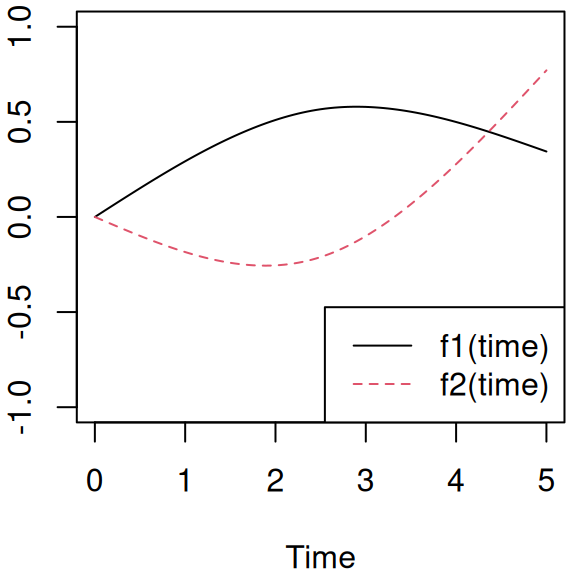
Figure 3.14: The two natural cubic spline basis functions, f1(time) and f2(time), used to model non-linear time trends.
These functions allow for flexible trajectories since they are associated to individual weights (i.e., fixed + random effects). The simulation process is a direct extension of the random slope model. We just define a 3x3 covariance matrix (instead of 2x2) and then use rmvnorm() to draw \(n\) vectors of realizations of the three random effects.
b_1f1=0# f1 fixed effectb_1f2=-2# f2 fixed effectb_2f1=2# f1 fixed effect x trtb_2f2=3# f2 fixed effect x trtb_slof1SD=0.5# random slope f1 standard deviationb_slof2SD=0.5# random slope f2 standard deviationcor_bintslof1=0.8# correlationscor_bintslof2=-0.5cor_bslof1slof2=-0.3cov_bintslof1 <- b_intSD*b_slof1SD*cor_bintslof1 # covariancescov_bintslof2 <- b_intSD*b_slof2SD*cor_bintslof2cov_bslof1slof2 <- b_slof1SD*b_slof2SD*cor_bslof1slof2Sigma2=matrix(c(b_intSD^2,cov_bintslof1,cov_bintslof2, cov_bintslof1,b_slof1SD^2,cov_bslof1slof2, cov_bintslof2,cov_bslof1slof2,b_slof2SD^2),ncol=3) # variance - covarianceMVnorm <-rmvnorm(n, rep(0, 3), Sigma2)b_int <-rep(MVnorm[,1], each=n_i)b_slof1 <-rep(MVnorm[,2], each=n_i)b_slof2 <-rep(MVnorm[,3], each=n_i)linPred <- b_0 + b_int + b_2*trt + (b_1f1 + b_slof1)*f1(time) + b_2f1*f1(time)*trt + (b_1f2 + b_slof2)*f2(time) + b_2f2*f2(time)*trtY <-rnorm(n_i*n, linPred, b_e) # observed outcomedatLME3 <-data.frame(id, time, Y, trt=as.factor(trt))summary(datLME3) # longitudinal dataset
       id              time           Y           trt
 Min.   :   1.0   Min.   :0.0   Min.   :-5.0267   0:3114
 1st Qu.: 250.8   1st Qu.:1.0   1st Qu.: 0.1669   1:2886
 Median : 500.5   Median :2.5   Median : 1.3694
 Mean   : 500.5   Mean   :2.5   Mean   : 1.3569
 3rd Qu.: 750.2   3rd Qu.:4.0   3rd Qu.: 2.5251
 Max.   :1000.0   Max.   :5.0   Max.   : 7.1013
We can have a look at the individual trajectories:
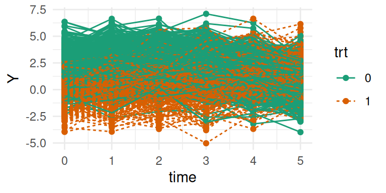
ggplot(datLME3, aes(time, Y, group = id, color = trt, linetype=trt)) +geom_point() +geom_line() +labs(color ="trt") +theme_minimal()
Figure 3.15: Simulated individual longitudinal trajectories from a model with random effects on splines, showing flexible, non-linear individual trajectories.
Individual trajectories can now be non-linear due to the inclusion of the splines. We can directly use the functions f1 and f2 in the formula to fit the model with INLAjoint:
M_lme3 <-joint(formLong = Y ~ (f1(time) +f2(time)) * trt + (1+f1(time) +f2(time)|id),id ="id", timeVar ="time", dataLong=datLME3)summary(M_lme3, sdcor=T)
Figure 3.16 shows the marginal posterior densities of the fixed effects and residual error:
plot(M_lme3)$Outcomes$L1
Figure 3.16: Posterior marginal distributions of the fixed effects and residual error variance from a spline-based mixed model. Dashed vertical red lines indicate the true values.
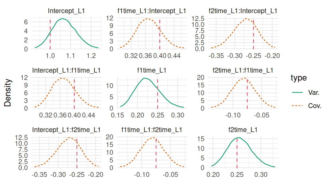
For the random effects, there are now 3 variance parameters and 3 covariance parameters, the plot of the marginal posterior for this variance-covariance matrix is included among the plots returned by the plot() function:
plot(M_lme3)$Covariances$L1
Figure 3.17: Posterior marginal distributions of the variance-covariance components for a spline-based random effects model. Dashed vertical red lines indicate the true values.
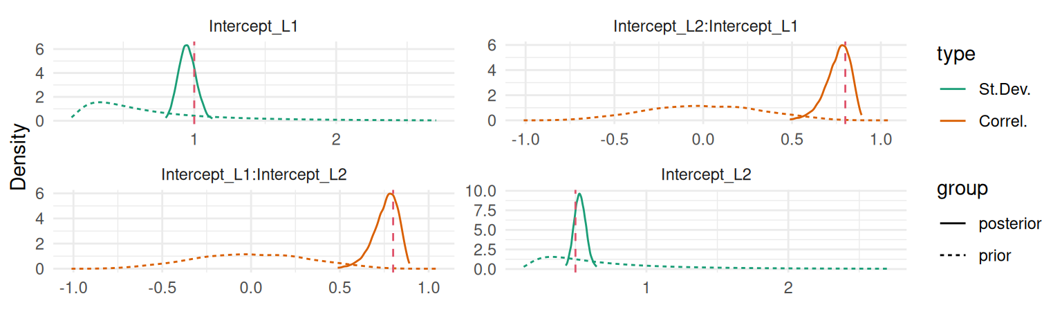
We can see how posteriors differ from priors with the argument priors=TRUE in the call of the plot() function that will add priors on top of posteriors:
plot(M_lme3, priors=TRUE)$Covariances$L1
Figure 3.18: Comparison of prior (dashed lines) and posterior distributions for the random effects variance-covariance components in a spline-based model.
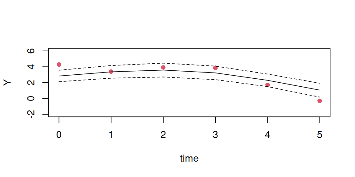
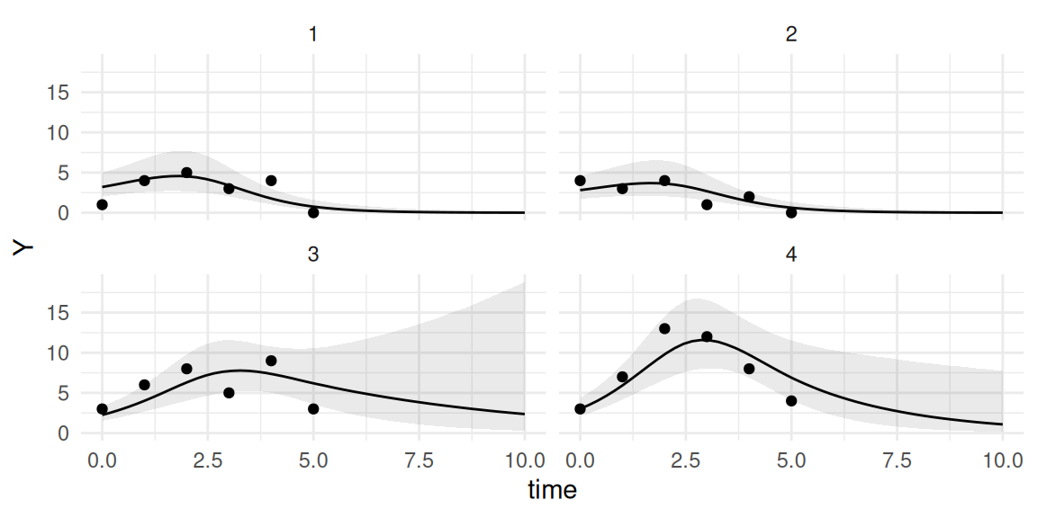
All the model parameters are fitted correctly since their posterior densities align with the true values. We can check the observed marker values and compare to the fitted linear predictor for the first individual:
Figure 3.19: Fitted individual trajectory for a subject from a spline-based random effects model, showing the observed data (points) and the fitted non-linear trajectory (solid line) with its 95% credible interval (dashed lines).
We see how the trajectory is now more flexible and can change trend over time. Now we may be interested in the derivation of predictions from this fitted model. We can simulate data for some new individuals and predict the underlying trajectory of the marker conditional on a few observations and the fitted model. First we simulate data for 4 new individuals:
npts <-1111# compute true values at many time pointsnind <-4# number of individualsntime=rep(seq(0, 10, len=npts), nind) # timentrt=rep(0:1, each=nind*npts/2) # trtMVnorm2 <-rmvnorm(nind, rep(0, 3), Sigma2) # sample random effectsnb_int <-rep(MVnorm2[,1], each=npts) # random interceptnb_slof1 <-rep(MVnorm2[,2], each=npts) # random f1nb_slof2 <-rep(MVnorm2[,3], each=npts) # random f2nlinPred <- b_0 + nb_int + b_2*ntrt + (b_1f1 + nb_slof1)*f1(ntime) + b_2f1*f1(ntime)*ntrt + (b_1f2 + nb_slof2)*f2(ntime) + b_2f2*f2(ntime)*ntrt # linear predictordatTrue <-data.frame(id=rep(1:nind, each=npts), time=ntime, Y=nlinPred, trt=as.factor(rep(0:1, each=nind*npts/2))) # trueNewData <- datTrue[datTrue$time %in%0:5,] NewData$Y <- NewData$Y +rnorm(nrow(NewData), sd=b_e)str(NewData) # observed data for prediction
'data.frame':   24 obs. of  4 variables:
 $ id  : int  1 1 1 1 1 1 2 2 2 2 ...
 $ time: num  0 1 2 3 4 5 0 1 2 3 ...
 $ Y   : num  0.249 1.413 1.343 0.592 -0.666 ...
 $ trt : Factor w/ 2 levels "0","1": 1 1 1 1 1 1 1 1 1 1 ...
Here we have 24 new observations corresponding to 4 individuals with 6 repeated measurements between time 0 and 5. We can predict the marker’s true trajectory (i.e., free from the residual error) at horizon 10 with the predict() function:
P <-predict(M_lme3, NewData, horizon=10)
Here, the predict function automatically defines 50 equidistant time points between 0 and horizon and evaluates the linear predictor for each new individual (i.e., using the posterior distribution of the random effects conditional on the new data) at these time points (note that in addition to these time points, the maximum measurement time of the marker provided in the new dataset is also included, which can be useful for comparisons of observed vs. fitted and particularly useful for predictive accuracy metrics computation for models that include survival components, see Chapter 4).
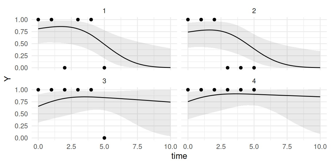
As discussed in Chapter 2, we can change the number of time points with the argument NtimePoints in the call of the predict() function and alternatively, a vector of fixed time points can be provided with the argument timePoints (see Section 1.5.5). We can check the fit of our 4 new individual’s observations and compare the estimated trajectory up to time 10 with the true underlying trajectory:
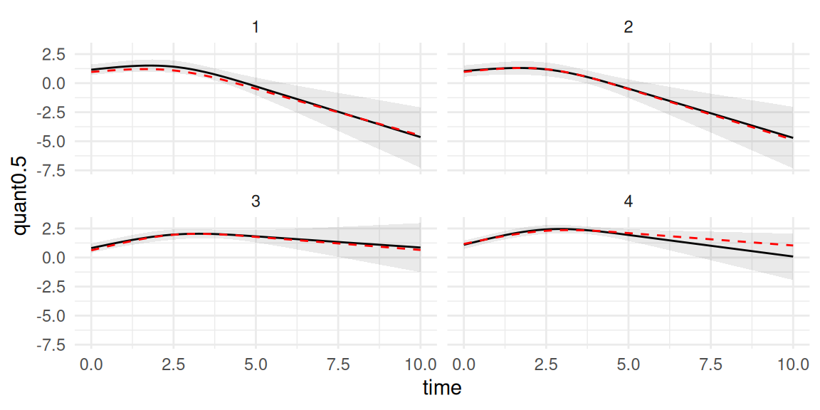
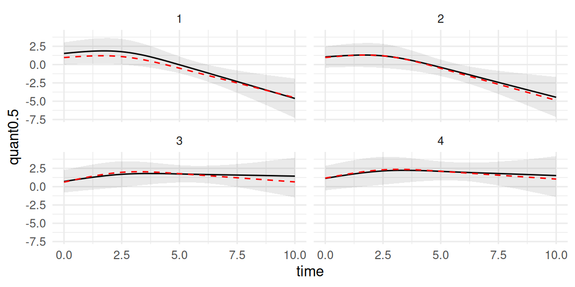
ggplot(P$PredL, aes(x = time, y = quant0.5)) +geom_line() +geom_ribbon(aes(ymin=quant0.025, ymax=quant0.975), alpha=0.1) +geom_point(data=NewData, aes(x=time, y=Y)) +ylab("Y") +theme(legend.position="none") +facet_wrap(~id) +theme_minimal()
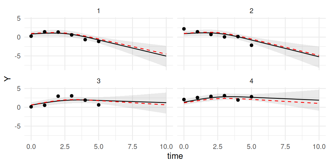
Figure 3.20: Predicted longitudinal trajectories for new subjects from a spline-based model. Each panel shows observed data (points), true trajectory (dashed red), posterior mean prediction (solid black), and the 95% credible interval for the true mean trajectory (shaded region).
The prediction plot displays the estimated trajectory for each new individual, conditional on their observed data. We can see that our predictions accurately capture the true underlying trajectory of the marker for the 4 individuals. The shaded region around the solid line represents the 95% credible interval. It answers the question: “Given the data and the model, what is the uncertainty about the true average value of the marker for this specific individual at each future time point?”. The uncertainty is therefore for the true value of the marker (i.e., free from residual error). If we are interested in the uncertainty over the observed values, we can get the 95% credible interval including the residual error term by setting the argument resErrLong=TRUE in the call of the predict() function:
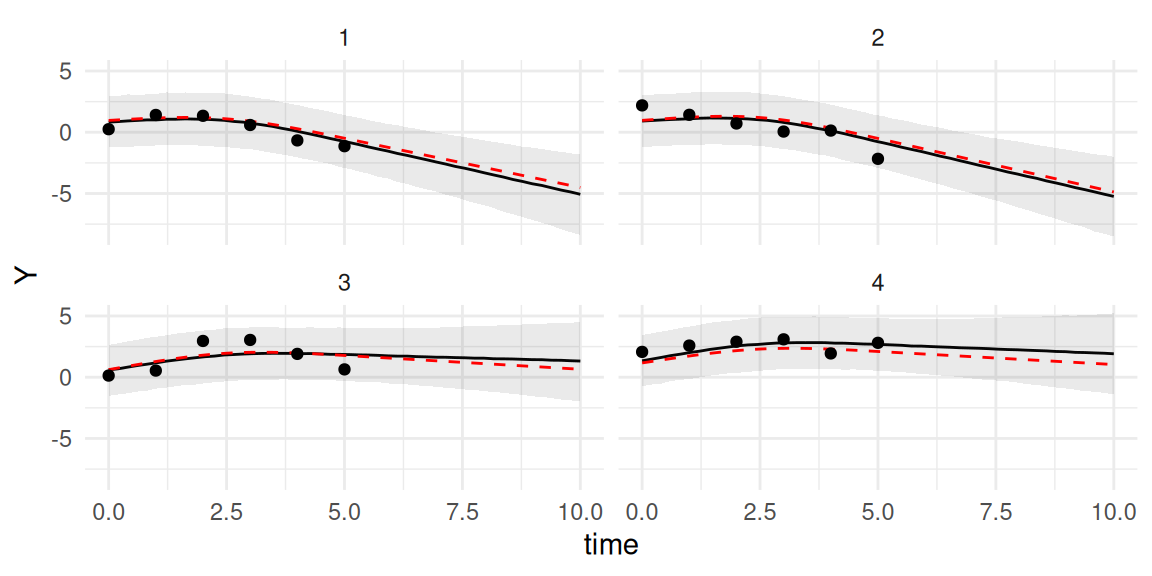
P <-predict(M_lme3, NewData, horizon=10, resErrLong =TRUE)ggplot(P$PredL, aes(x = time, y = quant0.5)) +geom_line() +geom_ribbon(aes(ymin=quant0.025, ymax=quant0.975), alpha=0.1) +geom_line(data=datTrue, aes(x=time, y=Y), linetype=2, color="red") +geom_point(data=NewData, aes(x=time, y=Y)) +ylab("Y") +theme(legend.position="none") +facet_wrap(~id) +theme_minimal()
Figure 3.21: Predicted longitudinal trajectories for new subjects from a spline-based model, with the 95% credible interval (shaded region) now including the residual error variance to represent uncertainty for observations.
Here the interval answers a different question: “If we were to take a new measurement for this individual, where would we expect 95% of those new observations to fall?”. This 95% credible interval is larger as it covers 95% of the observed values of the marker, while the previous one included 95% of the true values of the marker.
3.3 Generalized linear mixed-effects model
The linear mixed-effects model is limited to Gaussian distributed outcomes but as described in the introduction of this chapter, other types of distributions are encountered and require an appropriate methodology. The Generalized Linear Mixed-effects Model (GLMM) is a flexible generalization of ordinary linear mixed-effects model designed for response variables with non-Gaussian distributions. The distribution of the response variable is assumed to belong to the exponential family including Bernoulli, Binomial and Poisson distributions. The linear model is related to the response variable through a link function \(g(\cdot)\). Using the same notations as in previous section, the model is defined as \[\begin{align*}
g(\textrm{E}[Y_{i}(t)])&=X_{i}(t)^\top \beta+ Z_{i}(t)^\top b.
\end{align*}\]
As opposed to the linear mixed-effects model in Section 3.2, the calculation of the log-likelihood has no analytic solution and the integral over the random effects \(b\) is computed numerically in most cases (exceptions include, for example, the log-linear Poisson model with Gamma distributed random effects). The lack of analytical solution is due to the non-linear function \(g(\cdot)\) that links the linear predictor to the outcome. Numerical computation of the integral over the random effects complicates the computation of the likelihood, making the maximum likelihood estimation of GLMMs much more difficult than for the linear mixed model. With INLA, these models are treated similar to the linear mixed-effects model (due to the laplace approximation used whenever the likelihood is non-Gaussian) and minor differences in computation time are observed (Rustand et al. (2024)), making INLA a method of choice to fit this class of models under the latent Gaussian assumption. In the following we illustrate some of the available mixed-effects models for longitudinal data but since INLA is compatible with a large spectrum of likelihoods, the presentation is not fully exhaustive and more options are already available or could be implemented.
3.3.1 Poisson mixed-effects for a count outcome
We first introduce the Poisson mixed-effects model as one example of GLMM, designed to handle response variables that follow a Poisson distribution, which is particularly suitable for count data. The Poisson mixed-effects model incorporates both fixed and random effects, allowing for the inclusion of individual-specific variations in the count data. The link function typically used is the log link, which relates the linear predictor to the expected count. We can simulate data from this model by reusing the linear predictor simulated in the previous section, and applying the link function to sample from a Poisson distribution. The model is then defined as: \[\begin{align*}
\log(\textrm{E}[Y_{i}(t)])=&\beta_0 + b_{i0} + (\beta_1 + b_{i1})\cdot f_1(t) + (\beta_2 + b_{i2})\cdot f_2(t) + \\
&\beta_3\cdot trt_i + \beta_4\cdot trt_i\cdot f_1(t) + \beta_5\cdot trt_i\cdot f_2(t)
\end{align*}\] The key difference with the previous model is the inclusion of a link function and the absence of an additive residual error term. Unlike linear mixed-effects models for continuous outcomes, where we model the exact value of a continuous variable, the Poisson mixed-effects model focuses on the underlying Poisson rate that generates the observed counts. We can simulate count observations based on this model:
   Min. 1st Qu.  Median    Mean 3rd Qu.    Max.
   0.00    1.00    4.00   10.68   10.00  534.00
We can have a look at the simulated individual trajectories:
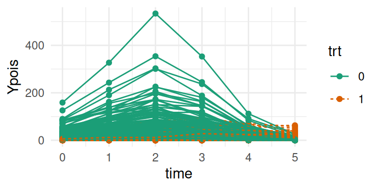
ggplot(datLME3, aes(time, Ypois, group = id, color = trt, linetype=trt)) +geom_point() +geom_line() +labs(color ="trt") +theme_minimal()
Figure 3.22: Simulated count data from a Poisson mixed-effects model showing individual trajectories over time, where colors and line type indicates treatment group.
We can see how the data is becoming difficult to visualize since the log link makes simulated counts reach high values. The call of the joint() function is very similar to the LME fitted in previous section, except that we need to change the family argument (which is a character string (or a vector for multivariate models) giving the name of families for the longitudinal outcomes) to set the “poisson” distribution:
We can check posterior marginals of the fixed effects:
plot(M_pois)$Outcomes$L1
Figure 3.23: Posterior marginal distributions of fixed effects for the Poisson mixed-effects model with true values depicted by dashed red lines.
And we can also check the posterior marginals of the random effects’s variance-covariance:
plot(M_pois)$Covariances$L1
Figure 3.24: Posterior marginal distributions of the random effects variance-covariance parameters for the Poisson mixed-effects model with true values depicted by vertical lines.
As observed with the LME, all the model parameters are recovered properly. We can also illlustrate how to perform individual predictions, based on the 4 individuals simulated in the previous section we can generate observed counts for these individuals and predict similarly:
We can compare our predicted trajectories for the rate of the Poisson distribution as shown in Figure 3.25:
ggplot(P$PredL, aes(x = time, y = quant0.5)) +geom_line() +geom_ribbon(aes(ymin=quant0.025, ymax=quant0.975), alpha=0.1) +theme(legend.position="none") +facet_wrap(~id) +theme_minimal()
Figure 3.25: Predicted trajectories for the rate of the Poisson distribution for 4 new individuals, with observed counts and true trajectories (dashed red lines) for comparison.
We can see that the model is predicting true trajectories accurately. We may however be more interested in the scale of the observed data since we are here looking at the predicted linear predictor. It allows for the comparison of observed data versus model predictions but requires to apply the inverse link function to the linear predictor. This can be done internally in order to directly have uncertainty on the transformed scale by including the argument inv.link=TRUE in the call of the predict() function. We can then directly compare observed counts vs. predicted Poisson rate:
P <-predict(M_pois, NewData, horizon=10, inv.link=TRUE)ggplot(P$PredL, aes(x = time, y = quant0.5)) +geom_line() +geom_ribbon(aes(ymin=quant0.025, ymax=quant0.975), alpha=0.1) +geom_point(data=NewData, aes(x=time, y=Ypois)) +ylab("Y") +theme(legend.position="none") +facet_wrap(~id) +theme_minimal()
Figure 3.26: Predicted Poisson expected counts for 4 new individuals with observed counts shown as points and 95% credible intervals shown as the shaded region.
We can see that the model is able to accurately capture the individual counts and can predict future values dynamically.
3.3.2 Mixed-effects models for binomial data
The binomial likelihood family is used for outcomes that represent the number of successes in a fixed number of trials. This distribution is characterized by two parameters: the number of trials \(n\) and the probability of success \(p\) in each trial. It is defined as:
\[P(X=k)=\begin{pmatrix} n \\ k\end{pmatrix} p^k(1-p)^{n-k}\] where \(\begin{pmatrix} n \\ k\end{pmatrix}\) is the binomial coefficient, representing the number of ways to choose \(k\) successes out of \(n\) trials.
3.3.2.1 Logistic mixed-effects model for a binary outcome
In the context of a logistic mixed-effects model, the probability of success \(p\) is modeled using a logit link function. This function relates the linear predictor to the probability of success. Let’s consider the following model: \[\begin{align*}
\textrm{logit}(\textrm{E}[Y_{i}(t)])&=\textrm{logit}(p_{i}(t))=\log\left(\frac{p_{i}(t)}{1-p_{i}(t)}\right)\\
&=\beta_0 + b_{i0} + (\beta_1 + b_{i1})\cdot f_1(t) + (\beta_2 + b_{i2})\cdot f_2(t) + \\
& \ \ \ \beta_3\cdot trt_i + \beta_4\cdot trt_i\cdot f_1(t) + \beta_5\cdot trt_i\cdot f_2(t)
\end{align*}\]
The logit link function transforms the linear predictor into a probability, ensuring that \(p_{i}(t)\) remains between 0 and 1.
The logistic mixed-effects model is designed for binary outcomes. The most commonly used link function is the logit link, which relates the linear predictor to the probability of the binary outcome, although some alternatives may be of interest, such as the probit link function. It is important to note that binary data is inherently less informative than count or continuous data. As a result, the same amount of data provides more uncertainty in the estimates, requiring larger sample sizes to achieve comparable precision.
As done in the previous section, we can simulate a binary outcome based on the linear predictors simulated in Section 3.2.5:
   Min. 1st Qu.  Median    Mean 3rd Qu.    Max.
 0.0000  0.0000  1.0000  0.7343  1.0000  1.0000
We can have a look at the simulated individual trajectories:
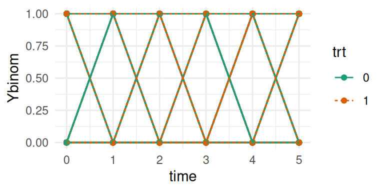
ggplot(datLME3, aes(time, Ybinom, group = id, color = trt, linetype=trt))+geom_point() +geom_line() +labs(color ="trt") +theme_minimal()
Figure 3.27: Simulated binary longitudinal data from a logistic mixed-effects model showing individual trajectories over time, colored by treatment group.
We can see that individuals may switch between 0 and 1 over time at measurement times (here all individuals have the same measurement times for simplicity).
Now we can fit the model with INLAjoint by simply switching the family to “binomial” from the previous call:
Figure 3.28 shows the posterior marginals for the fixed effects:
plot(M_binom)$Outcomes$L1
Figure 3.28: Posterior marginal distributions of fixed effects for the binomial mixed-effects model with true values depicted by dashed red lines.
And we can also check the posterior marginals for the random effects’s variance-covariance:
plot(M_binom)$Covariances$L1
Figure 3.29: Posterior marginal distributions of the random effects variance-covariance parameters for the binomial mixed-effects model with true values depicted by vertical lines.
The model fits well all parameters. We can use this model for predictions, starting by simulating observed counts for 4 new individuals (i.e., not used to fit the model) as introduced in the previous sections, and we can predict the true underlying individual linear predictor based on their observations:
We can compare our predictions for the individual linear predictor trajectories with the true trajectories as shown in Figure 3.30:
ggplot(P$PredL, aes(x = time, y = quant0.5)) +geom_line() +geom_ribbon(aes(ymin=quant0.025, ymax=quant0.975), alpha=0.1) +theme(legend.position="none") +facet_wrap(~id) +theme_minimal()
Figure 3.30: Predicted individual linear predictor trajectories for 4 new subjects from the binomial mixed-effects model, compared with true trajectories (dashed red lines).
The model is doing well and recovers the true underlying trajectories that generated the observed data for the new individuals. We can compare observed data with the probability of 1 vs. 0 by using the argument inv.link=TRUE in the call of the predict() function, which applies the inverse link function as discussed in previous sections.
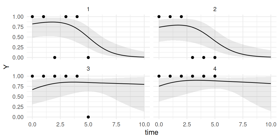
P <-predict(M_binom, NewData, horizon=10, inv.link=TRUE)ggplot(P$PredL, aes(x = time, y = quant0.5)) +geom_line() +geom_ribbon(aes(ymin=quant0.025, ymax=quant0.975), alpha=0.1) +geom_point(data=NewData, aes(x=time, y=Ybinom)) +ylab("Y") +theme(legend.position="none") +facet_wrap(~id) +theme_minimal()
Figure 3.31: Predicted probabilities of 1 vs. 0 for 4 new subjects from the binomial mixed-effects model using the inverse link function, with observed binary outcomes shown as points.
We can see in this figure how the model predicts the probability of 1 vs. 0 over time for each individual.
The link function associated to the families for the longitudinal outcomes can be modified with the link argument, which is a character string (or a vector for multivariate longitudinal outcomes). The various links available for a given family can be displayed in R with the following command after loading the INLA library: inla.doc("FAMILY NAME"). The link should be a vector of the same size as the family parameter and should be set to "default" for default (“identity” for gaussian, “log” for poisson, “logit” for binomial, etc.).
Here, the default link for binomial family is the logit link but we can switch for the probit link as follows:
We can compute the same individual predictions with this new link function:
P <-predict(M_binom2, NewData, horizon=10, inv.link=TRUE)ggplot(P$PredL, aes(x = time, y = quant0.5)) +geom_line() +geom_ribbon(aes(ymin=quant0.025, ymax=quant0.975), alpha=0.1) +geom_point(data=NewData, aes(x=time, y=Ybinom)) +ylab("Y") +theme(legend.position="none") +facet_wrap(~id) +theme_minimal()
Figure 3.32: Predicted probabilities for 4 new subjects from the binomial mixed-effects model using the probit link function, with observed binary outcomes shown as points.
We can see that this model gives a roughly similar predictions as the model with a logit link but with higher uncertainty, likely the consequence of using the wrong link (since we simulated from the logit).
3.3.2.2 Binomial mixed-effects model for proportions
The binomial family can also be used for proportion data where the outcome is the number of successes out of a fixed number of trials. Then, the number of trials can be displayed in the argument Ntrials in the control options of the joint() function. For example we can simulate from a binomial with 10 trials:
Here the binomial data is much more informative than binary (values between 0 and 10) and thus the model performs well and recovers all true parameters values. We only presented the Poisson mixed-effects model and the binomial mixed-effects model in the context of GLMMs but as explained in the introduction, many likelihoods are available and switching between likelihoods is simply done by changing the family of the model. Here are some of the available likelihood families among more than 100 options supported by R-INLA:
Gamma (gamma) for positive continuous data.
Beta (beta) for continuous data bounded between 0 and 1.
Negative Binomial (nbinomial) for overdispersed count data.
Beta-Binomial (betabinomial) for overdispersed binary or proportion data.
Censored Poisson (cenpoisson) for censored count data.
Censored Negative Binomial (cennbinomial) for censored overdispersed count data.
3.4 Multivariate longitudinal outcomes
It is common to observe multiple longitudinal outcomes of interest in the same study. We could be interested in the relationship between markers or take advantage of their correlation to enhance their analysis. Let’s consider we observe one continuous outcome along with a count outcome and a binary outcome, we may want to fit the following model:
\[\begin{align*}
\textrm{E}[Y_{1i}(t)]=&\beta_{10} + b_{i10} + \beta_{11}\cdot f_1(t) + \beta_{12}\cdot f_2(t) + \\
&\beta_{13}\cdot trt_i + \beta_{14}\cdot trt_i\cdot f_1(t) + \beta_{15}\cdot trt_i\cdot f_2(t)\\
\log(\textrm{E}[Y_{2i}(t)])=&\beta_{20} + b_{2i0} + \beta_{21}\cdot f_1(t) + \beta_{22}\cdot f_2(t) + \\
&\beta_{23}\cdot trt_i + \beta_{24}\cdot trt_i\cdot f_1(t) + \beta_{25}\cdot trt_i\cdot f_2(t)\\
\textrm{logit}(\textrm{E}[Y_{3i}(t)])=&\beta_{30} + b_{3i0} + \beta_{31}\cdot f_1(t) + \beta_{32}\cdot f_2(t) + \beta_{33}\cdot trt_i + \\
&\beta_{34}\cdot trt_i\cdot f_1(t) + \beta_{35}\cdot trt_i\cdot f_2(t)
\end{align*}\] where fixed effects \(\beta_{k}\) corresponds to outcome \(k = 1, 2, 3\) for the continuous, count and binary outcomes, respectively. The random effects \(b_{ki}\) considered here are only random intercepts for simplicity, for outcome \(k\) and individual \(i\). The continuous outcome also includes an additive Gaussian residual error term as in Section 3.2.3. We can simulate data from this model:
As discussed in Section 2.8, multiple outcomes can be fitted simultaneously with INLA with a specific data format. First we need to have unique ids for the 3 correlated random intercepts, we also need to make unique columns for each fixed effect and then we can create a dataset for the trivariate outcome using the inla.rbind.data.frames function (note that this step is to prepare the data in the R-INLA format and is only presented for transparency and clarity on the use of R-INLA, however this is all done automatically and internally with INLAjoint as illustrated later in this section):
datLME3$id2 <- datLME3$id +max(datLME3$id) # id random for outcome 2datLME3$id3 <- datLME3$id +max(datLME3$id)*2# id random for outcome 3datLME3$time2 <- datLME3$time # time outcome 2datLME3$time3 <- datLME3$time # time outcome 3datLME3$trt2 <- datLME3$trt # trt outcome 2datLME3$trt3 <- datLME3$trt # trt outcome 3datLME3$int <- datLME3$int2 <- datLME3$int3 <-1# interceptsdata_MULT <-inla.rbind.data.frames( datLME3[, c("id", "int", "time", "trt", "Y3")], datLME3[, c("id2", "int2", "time2","trt2", "Ypois3")], datLME3[, c("id3", "int3", "time3","trt3", "Ybinom3")])
We can see the data structure by looking at the first individual data:
data_MULT[which(data_MULT$id==1|# id 1 data_MULT$id2==1+max(datLME3$id) | data_MULT$id3==1+max(datLME3$id)*2), -c(1:2,6:7,11:12)]
      time  trt         Y3 time2 trt2 Ypois3 time3 trt3 Ybinom3
1        0    1 -1.6613414    NA <NA>     NA    NA <NA>      NA
2        1    1 -0.4502668    NA <NA>     NA    NA <NA>      NA
3        2    1 -1.1054801    NA <NA>     NA    NA <NA>      NA
4        3    1  1.6171885    NA <NA>     NA    NA <NA>      NA
5        4    1  0.5708752    NA <NA>     NA    NA <NA>      NA
6        5    1 -0.3965601    NA <NA>     NA    NA <NA>      NA
6001    NA <NA>         NA     0    1      0    NA <NA>      NA
6002    NA <NA>         NA     1    1      0    NA <NA>      NA
6003    NA <NA>         NA     2    1      0    NA <NA>      NA
6004    NA <NA>         NA     3    1      3    NA <NA>      NA
6005    NA <NA>         NA     4    1      0    NA <NA>      NA
6006    NA <NA>         NA     5    1      4    NA <NA>      NA
12001   NA <NA>         NA    NA <NA>     NA     0    1       0
12002   NA <NA>         NA    NA <NA>     NA     1    1       1
12003   NA <NA>         NA    NA <NA>     NA     2    1       0
12004   NA <NA>         NA    NA <NA>     NA     3    1       1
12005   NA <NA>         NA    NA <NA>     NA     4    1       1
12006   NA <NA>         NA    NA <NA>     NA     5    1       0
The data involves one line for the contribution to each likelihood at each time point, such that the first 6 lines are for the Gaussian submodel, the next 6 lines are for the Poisson submodel while the last 6 lines are for the Logistic submodel. In order to fit the model with INLA, we must combine the 3 outcomes to form one multivariate outcome. This can be done by setting the outcome as a data frame with three columns:
List of 13
 $ id    : int [1:18000] 1 1 1 1 1 1 2 2 2 2 ...
 $ id2   : int [1:18000] NA NA NA NA NA NA NA NA NA NA ...
 $ id3   : num [1:18000] NA NA NA NA NA NA NA NA NA NA ...
 $ int   : num [1:18000] 1 1 1 1 1 1 1 1 1 1 ...
 $ int2  : num [1:18000] NA NA NA NA NA NA NA NA NA NA ...
 $ int3  : num [1:18000] NA NA NA NA NA NA NA NA NA NA ...
 $ time  : num [1:18000] 0 1 2 3 4 5 0 1 2 3 ...
 $ time2 : num [1:18000] NA NA NA NA NA NA NA NA NA NA ...
 $ time3 : num [1:18000] NA NA NA NA NA NA NA NA NA NA ...
 $ trt   : Factor w/ 2 levels "0","1": 2 2 2 2 2 2 2 2 2 2 ...
 $ trt2  : Factor w/ 2 levels "0","1": NA NA NA NA NA NA NA NA NA NA ...
 $ trt3  : Factor w/ 2 levels "0","1": NA NA NA NA NA NA NA NA NA NA ...
 $ Yjoint:'data.frame': 18000 obs. of  3 variables:
  ..$ Y3     : num [1:18000] -1.661 -0.45 -1.105 1.617 0.571 ...
  ..$ Ypois3 : int [1:18000] NA NA NA NA NA NA NA NA NA NA ...
  ..$ Ybinom3: int [1:18000] NA NA NA NA NA NA NA NA NA NA ...
Now we need to setup the functions of time, then we can call the inla() function to fit the model:
Time used:
    Pre = 0.511, Running = 14, Post = 0.411, Total = 15
Fixed effects:
                mean     sd 0.025quant 0.5quant 0.975quant   mode kld
int            0.668 18.257    -35.133    0.668     36.469  0.668   0
f1time         0.035  0.094     -0.150    0.035      0.220  0.035   0
f2time        -2.016  0.052     -2.118   -2.016     -1.914 -2.016   0
trt0           1.359 18.257    -34.441    1.359     37.160  1.359   0
trt1          -0.692 18.257    -36.493   -0.692     35.109 -0.692   0
int2           2.051  0.025      2.003    2.051      2.099  2.051   0
f1time2       -0.062  0.031     -0.123   -0.062     -0.001 -0.062   0
f2time2       -2.031  0.028     -2.086   -2.031     -1.976 -2.031   0
trt21         -2.024  0.049     -2.120   -2.024     -1.928 -2.024   0
int3           1.783  0.115      1.557    1.783      2.009  1.783   0
f1time3        0.390  0.273     -0.145    0.390      0.926  0.390   0
f2time3       -2.004  0.128     -2.255   -2.004     -1.753 -2.004   0
trt31         -1.751  0.143     -2.032   -1.751     -1.470 -1.751   0
f1time:trt1    1.999  0.136      1.731    1.999      2.266  1.999   0
f2time:trt1    3.009  0.075      2.862    3.009      3.156  3.009   0
f1time2:trt21  2.036  0.083      1.873    2.036      2.198  2.036   0
f2time2:trt21  3.042  0.040      2.963    3.042      3.120  3.042   0
f1time3:trt31  1.382  0.340      0.715    1.382      2.049  1.382   0
f2time3:trt31  2.680  0.177      2.334    2.680      3.027  2.680   0

Random effects:
  Name    Model
    id IIDKD model
   id2 Copy
   id3 Copy

Model hyperparameters:
                                          mean    sd 0.025quant 0.5quant 0.975quant   mode
Precision for the Gaussian observations  0.972 0.019      0.934    0.972      1.011  0.972
Theta1 for id                            0.849 0.100      0.653    0.848      1.048  0.846
Theta2 for id                            0.869 0.061      0.744    0.870      0.985  0.876
Theta3 for id                            0.979 0.121      0.742    0.979      1.219  0.977
Theta4 for id                           -3.126 0.340     -3.834   -3.114     -2.497 -3.055
Theta5 for id                            2.717 0.767      1.179    2.726      4.200  2.766
Theta6 for id                            1.341 0.455      0.414    1.352      2.204  1.399

Marginal log-Likelihood:  -25780.98
 is computed
Posterior summaries for the linear predictor and the fitted values are computed
(Posterior marginals needs also 'control.compute=list(return.marginals.predictor=TRUE)')
The output from R-INLA does not consider outcomes as separate and the summary is still structured as fixed effects and hyperparameters grouped together (while we will see later in this section that INLAjoint has a more convenient structure for the output of multi-outcome models). In the summary, we can see that each outcome’s fixed effects are estimated well and returns similar results as univariate models fitted before. For the multivariate random effects, they are parameterized with the Cholesky of the precision matrix (i.e., inverse of variance-covariance), which is more stable and efficient numerically compared to other parametrizations such as precision and correlations, but cannot be interpreted directly. We need to sample from these parameters in order to get summary statistics over the variance-covariance of the random effects as done in Section 3.2.4:
We can then get summary statistics over these samples (note that standard deviations and correlations can be obtained by setting the argument return.cov=FALSE when sampling) and compare to the true values used for data generation:
We can see that the fit is good for the first two random effects but the variance of the third random intercept is underestimated (c.f., last line), this could be related to R-INLA’s default priors which is Inverse Wishart for multivariate random effects. Given the low-informative binary data for the third outcome and the default INLA priors that shrinks quite heavily toward zero the variance components, we end-up with a lower value compared to the true value. We can change the prior for a more suitable option, such as INLAjoint’s default prior (see Section 3.10):
Now all the results are matching with true values. This illustrates how INLAjoint is tailored for these models by defining default priors that behave better than the strict (more stable numerically) priors used by default in R-INLA that may affect the results when the data is not sufficiently informative to overcome prior’s information. More details are given in Section 3.10.
While the data preparation is not complex, fitting multi-outcomes models with R-INLA can easily become an error-prone, cumbersome task. The use of INLAjoint for multivariate outcomes is much more user-friendly since all the data preparation is done internally. We can fit the same model with the following call, where the formula is a list of three formulas for each submodel and the family is a vector of the three corresponding families. The corLong argument is a boolean (default is FALSE) that is only used when multiple longitudinal outcomes are included. When set to TRUE, the correlation structure between random effects accross longitudinal markers is unspecified, while random effects accross longitudinal markers are assumed independent when this is set to FALSE (i.e., block-diagonal correlation structure of the random effects):
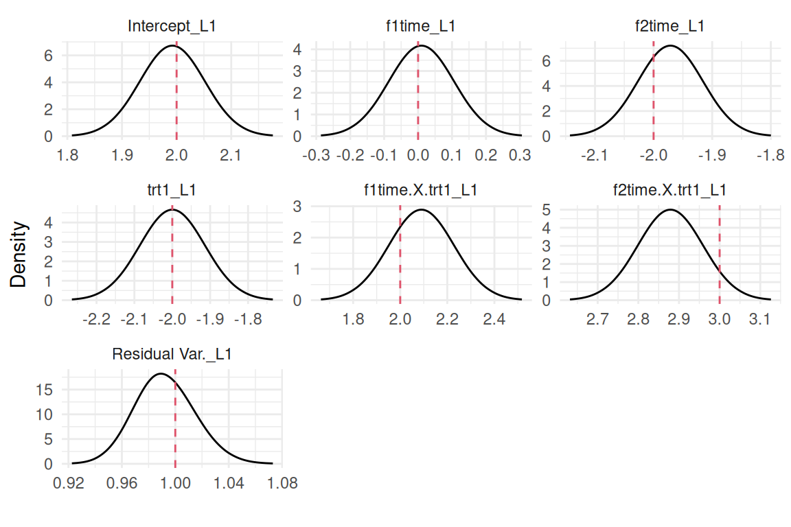
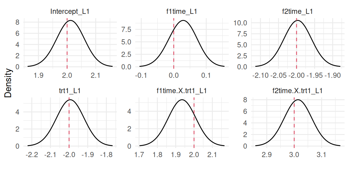
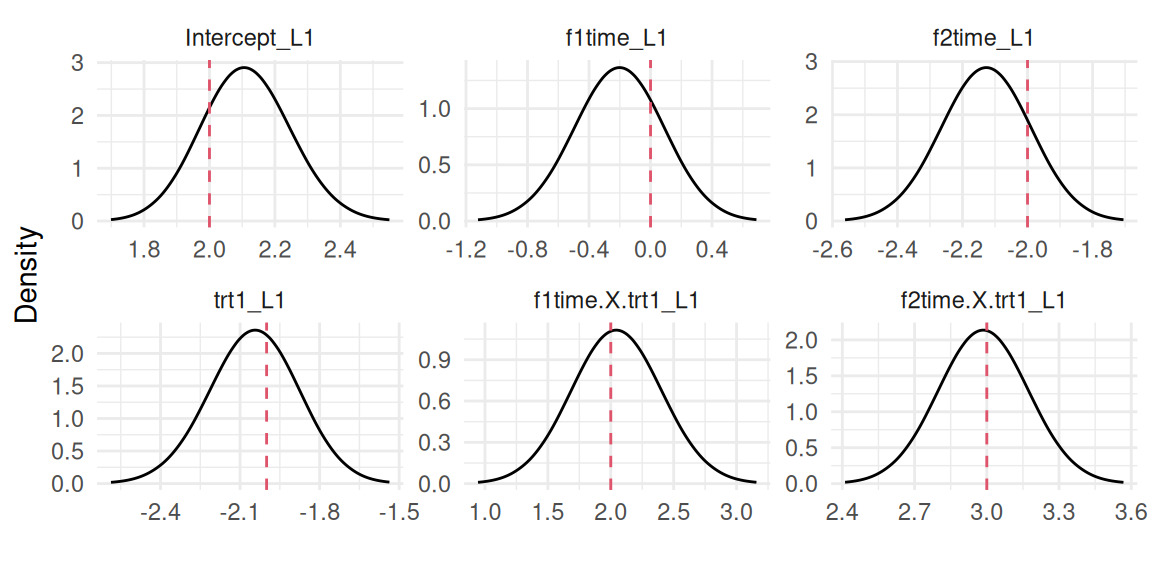
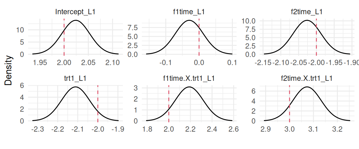
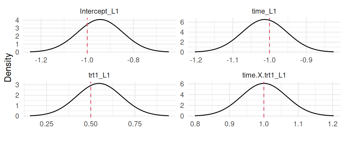
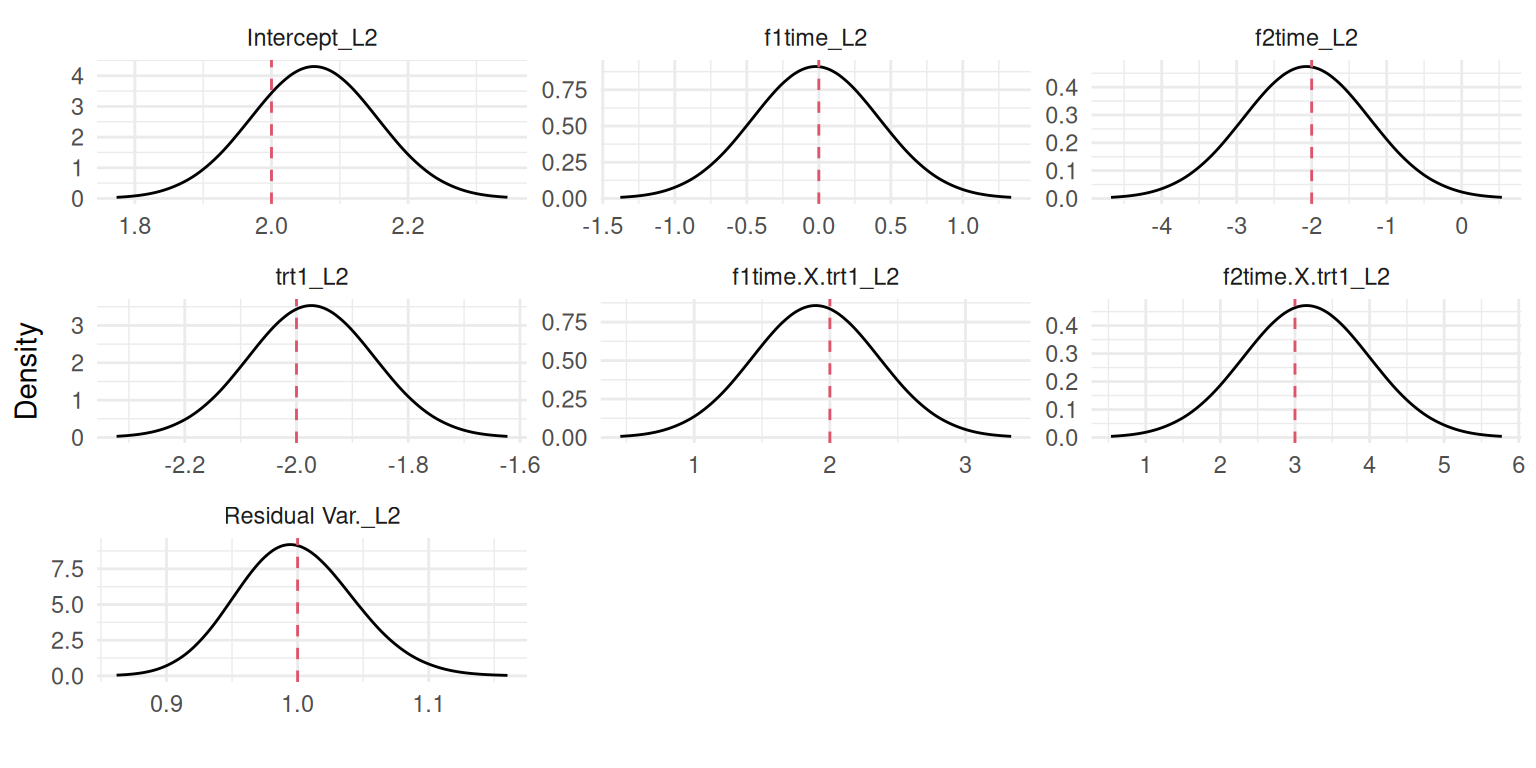
The output is more user-friendly compared to R-INLA’s output since we have all the fixed effects and likelihood parameters of each outcomes grouped together and the variance-covariance of the random effects given directly instead of the internally used Cholesky of the precision matrix. The interpretation of this model has two aspects: the effect of covariates (such as treatment) on each outcome, and the underlying relationships between the outcomes captured by the random effects structure. All the fixed effects and hyperparameters’s posterior marginals can be plotted with the plot() function, for example the variance-covariance of the random effects:
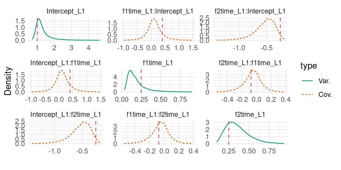
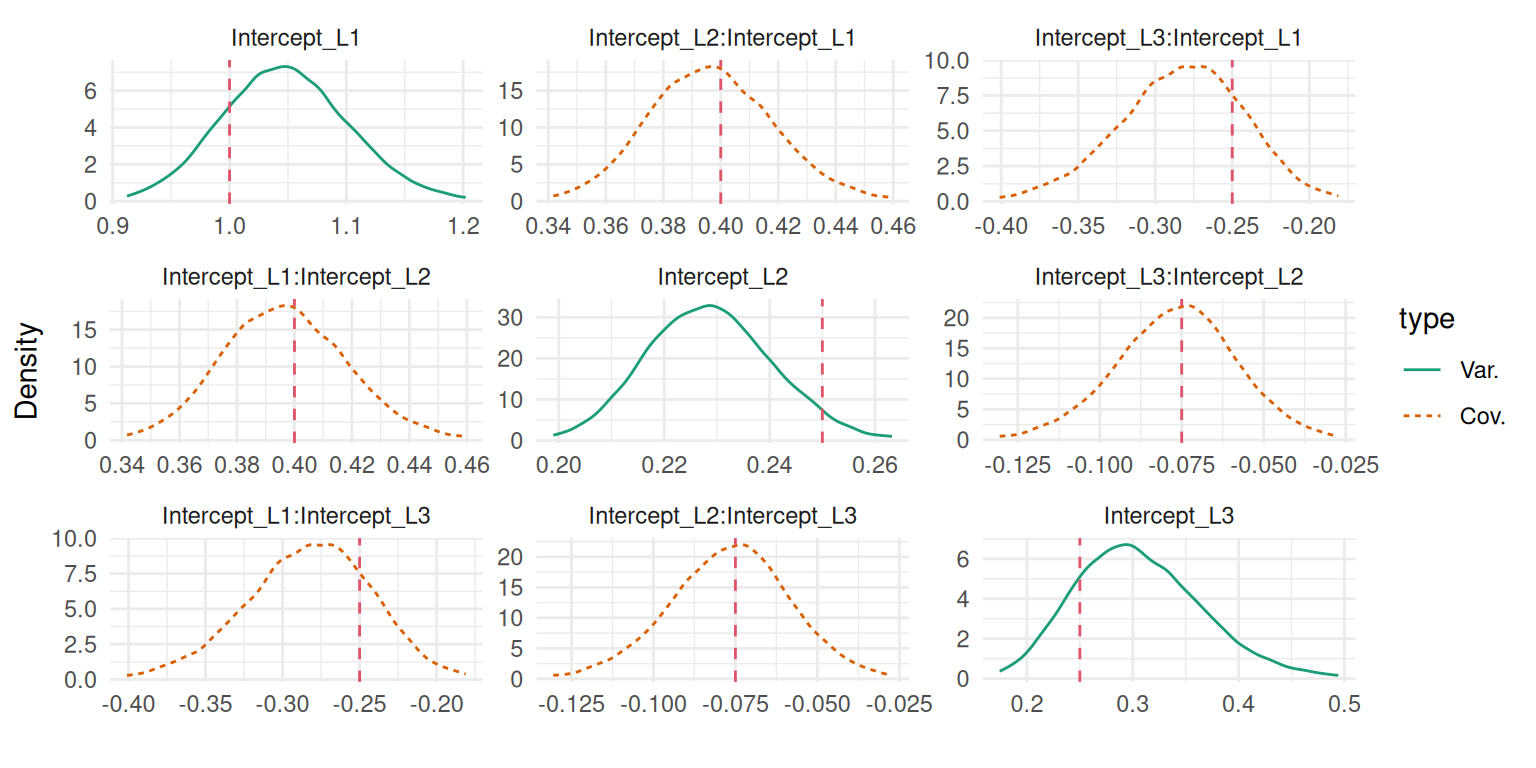
plot(M_multi3)$Covariances$L1
Figure 3.33: Posterior marginal distributions of the variance-covariance parameters for the multivariate mixed-effects model with true values depicted by dashed red lines.
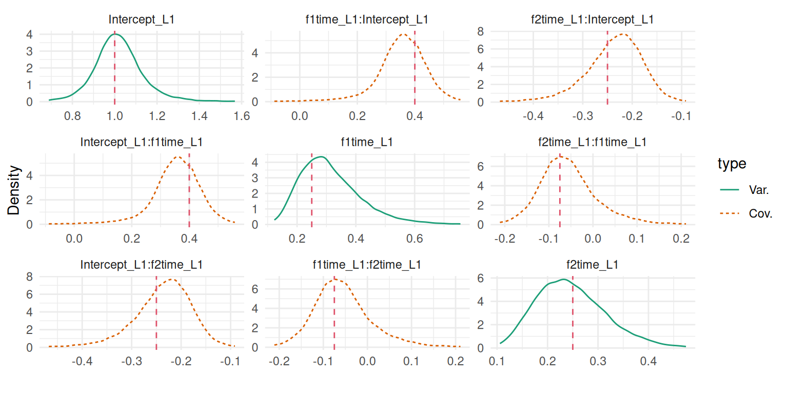
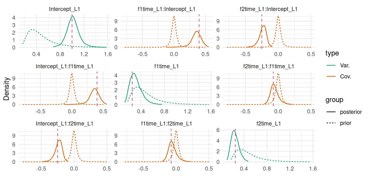
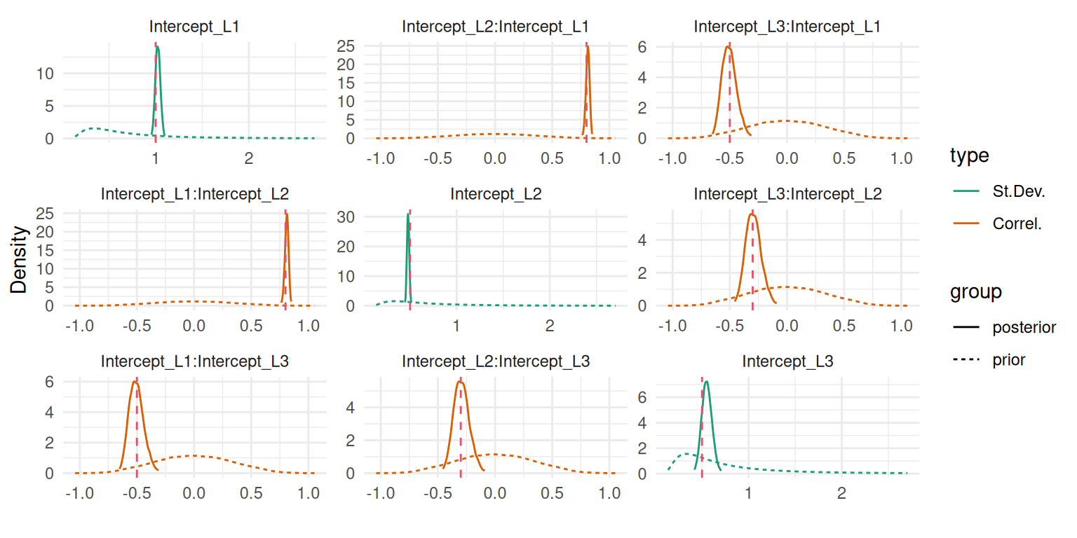
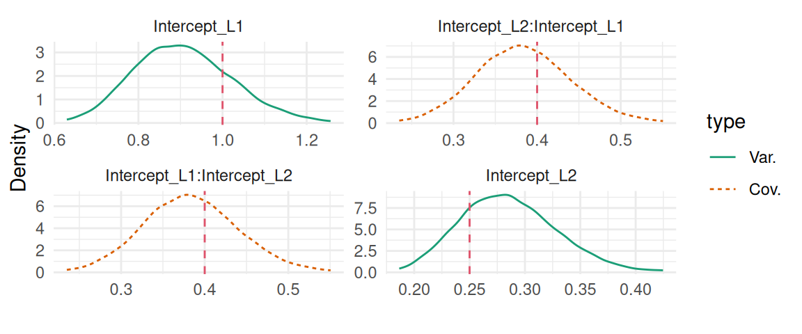
We can convert the variance-covariance to standard deviations and correlations in both the summary() and plot() functions by adding the argument sdcor=TRUE, and we can add prior distributions on top of posteriors in the plots by adding the argument priors=TRUE:
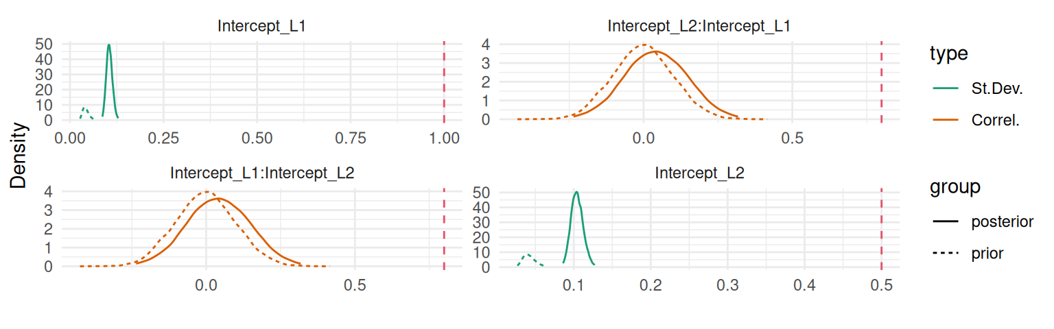
plot(M_multi3, sdcor=T, priors=T)$Covariances$L1
Figure 3.34: Posterior marginal distributions of the standard deviations and correlations for the multivariate mixed-effects model, with prior distributions shown as dashed curves and true values depicted by vertical red lines.
When multiple longitudinal outcomes are included in an INLAjoint model, it is possible to supply only one dataset assuming all the variables from all formulas are present in this dataset and it is also possible to provide a list of datasets specific for each outcome (in the same order as the list of formulas).
We can illustrate the use of the argument corLong by switching it to FALSE such that the 3 random intercepts from the previously fitted model are assumed independent:
Now the random effects are separated in the summary, each one associated to its outcome and we do not consider correlation between the longitudinal outcomes. This is the same as fitting these outcomes separately since there are no links anymore between the outcomes, but this could be relevant in the context of joint modeling where multiple independent longitudinal markers are assumed to affect the risk of one or multiple events.
3.5 Zero inflated mixed-effects models for count outcomes
Zero-inflated (ZI) mixed-effects models are used to handle count data that exhibit an excess of zeros beyond what is expected from standard count distributions, such as the Poisson or negative binomial. In many applications, count data include a substantial number of zero observations. These zeros can arise from two distinct processes: “structural zeros” are zeros present in excess while “sampling zeros” (or “random zeros”) are zeros that occur naturally as part of the distribution. ZI models address this issue by combining two components: a zero-inflation component that models the excess zeros and a count component that models the counts. The zero-inflation component typically uses a binary model, such as a logistic or probit regression, to predict the probability of observing a zero count. The count component, on the other hand, employs a standard count distribution, such as the Poisson or negative binomial, to model the positive counts. When only structural zeros are considered, truncated-at-zero counts distributions can be used such that only non-zeros counts are modeled with the count distribution.
The zero-inflated mixed-effects model can be formally expressed as a mixture of two distributions. Let \(Y_{i}(t)\) represent the count outcome for individual \(i\) at time \(t\). We first introduce the simple case where the probability of zero is constant and then discuss more advanced settings for this probability. The model can be written as: \[ P(Y_{i}(t) = y) =
\begin{cases}
\pi + (1-\pi)e^{-\lambda_{i}(t)} & \text{if } y = 0 \\
(1-\pi)\frac{e^{-\lambda_{i}(t)}\lambda_{i}(t)^y}{y!} & \text{if } y > 0
\end{cases}\] where \(\pi\) is the probability of observing a structural zero, modeled with a logit link: \[\text{logit}(\pi) = \theta\] and \(\lambda_i(t)\) is the rate of the Poisson distribution, defined as: \[\log(\lambda_i(t)) = X_{i}(t)^\top \beta_1 + Z_{i}(t)^\top b_{1i}\]
If we only want to consider structural zeros, then we use the truncated-at-zero Poisson distribution instead of the standard Poisson: \[ P(Y_{i}(t) = y) =
\begin{cases}
\pi & \text{if } y = 0 \\
(1-\pi)\frac{e^{-\lambda_{i}(t)}\lambda_{i}(t)^y}{y!} & \text{if } y > 0
\end{cases}\]
We can simulate data from this model, assuming the truncated-at-zero Poisson distribution with zero-probability \(\pi=0.4\):
Then we can fit the model, using the family zeroinflatedpoisson0 which corresponds to the truncated-at-zero Poisson distribution (while zeroinflatedpoisson1 would correspond to the standard Poisson distribution):
We can see among the results that the new parameter for the probability of zero is accurately estimated (true value: 0.4). The variance of the random effect is also recovered well by the model (true value: 0.25) and all the fixed effects:
plot(M_zip)$Outcomes$L1
Figure 3.35: Posterior marginal distributions of fixed effects for the zero-inflated Poisson model with true values depicted by vertical lines.
When there is interest in fitting the probability \(\pi\) as a function of fixed effects (and possibly random effects), the model is slightly more complex: \[ P(Y_{i}(t) = y) =
\begin{cases}
\pi_i(t) + (1-\pi_i(t))e^{-\lambda_{i}(t)} & \text{if } y = 0 \\
(1-\pi_i(t))\frac{e^{-\lambda_{i}(t)}\lambda_{i}(t)^y}{y!} & \text{if } y > 0
\end{cases}\] where \(\pi_i(t)\) is the probability of observing a structural zero for individual \(i\) at time \(t\), modeled through a logistic regression: \[\text{logit}(\pi_{i}(t)) = X_{i}(t)^\top \beta_2 + Z_{i}(t)^\top b_{2i}\]
To fit this model, a different family must be used with INLA and the setup is slightly more involved, we show an example of this model in the following. Of note, to be compatible with the INLA framework, random effects can only be included in one of the linear predictors, either to fit the probability of zeros or to fit the counts distribution, the other linear predictor is then only composed of fixed effects.
The Poisson distribution assume that the mean and variance are equal, which is often a reasonable assumption but may not be suitable in all situations. For example if we consider the number of daily hospital admissions for a rare disease, the variance in admissions may be higher than the average due to occasional outbreaks or clustering of cases. The negative binomial distribution extends the Poisson to accommodate overdispersion, where the variance exceeds the mean. It is available in INLAjoint for zero-inflated data as the zeroinflatednbinomial0 likelihood for the truncated-at-zero distribution and zeroinflatednbinomial1 for the standard distribution.
The binomial distribution handles binary or proportion data, assuming a fixed number of trials and a constant probability of success, it is available for zero-inflated data as the zeroinflatedbinomial0 family for the truncated-at-zero distribution and zeroinflatedbinomial1 for standard binomial distribution The beta-binomial distribution extends the binomial by allowing the success probability to vary according to a Beta distribution, making it suitable for proportion data with overdispersion. It is available in INLAjoint as the zeroinflatedbetabinomial0 family for the truncated-at-zero distribution and zeroinflatedbetabinomial1 family for the standard distribution. More details on these families available by running the command inla.doc("zeroinflated") in R after loading the R-INLA library.
Let’s now get back to the zero inflated Poisson example, but we consider that the probability of 1 vs. 0 depends on a linear predictor, for example the covariate trt could have an effect on this probability: \[\text{logit}(\pi_{i}(t)) = \beta_2\cdot trt_i\]
Proba_i <-1/(1+exp(1-1.5*trt)) # probability of zeroB2 <-rbinom(nrow(datLME3), size=1, prob=Proba_i)datLME3$Ypois5 <-ifelse(B2==0, datLME3$Ypois3, 0)
In order to fit this model, we need to adapt the outcome to set it as a multi-column outcome where the first two columns are for the Poisson distribution (offset and observations, respectively) and the rest are predictors for the probability of zero, here we consider the intercept and trt effect (see inla.doc("0poisson") for additional details on this likelihood). We use the “build only” option introduced in Section 1.5.8 to first build the model and then switch the outcome to allow for covariates effect on the zero inflation probability:
E <-rep(1, length(datLME3$Ypois3)) # offset for Poisson log-rateint_p <-rep(1, length(datLME3$Ypois3))trt_p <- datLME3$trtY_ZI <-inla.mdata(cbind(datLME3$Ypois5, E), cbind(int_p, trt_p))M_zip20 <-joint(formLong =list( Y ~ (f1(time) +f2(time)) * trt + (1|id)),family="0poisson",id ="id", timeVar ="time", dataLong=datLME3, run=F)M_zip20$.args$data$Yjoint <- Y_ZIM_zip2 <-joint.run(M_zip20)summary(M_zip2)
Now the model includes two parameters for the logistic regression that quantifies the effect of covariates on the probability of 1 vs. 0, where beta1 is the fixed intercept and beta2 is the effect of treatment. Other fixed effects such as time could be included but the current parametrization does not allow for random effects (unless only fixed effects are included in the Poisson part, see `inla.doc(“0poisson”) for additional details). For hurdle models, it is also possible to define two submodels linked by shared or correlated random effects, similar to the approach for a semicontinuous outcome described in the next section.
3.6 Two-part mixed-effects models for semicontinuous outcomes
A semicontinuous distribution is characterized by a continuous distribution with a point mass. It is ususally a half-bounded interval where in most cases, the distribution has a lower bound at zero resulting in either a positive value or a zero. Such distributions are common, examples include medical costs (Duan et al. (1983), Liu et al. (2010)), alcohol consumption (Liu et al. (2008), Liu et al. (2016), Han et al. (2019)), gene expression data (McDavid et al. (2013), Finak et al. (2015)) or microbiome compositional data (Chen & Li (2016), Chai et al. (2018)). Semicontinuous distributions often arise when quantifying some exposure or measuring symptoms of a disease that may disappear. For example, repeated measurements of tumor size in cancer clinical trials can have a semicontinuous distribution when some patients have their tumors shrinking towards zero under treatment effect.
An illustration of the distribution of the repeated measurements of tumor size in a randomized clinical trial is presented in Figure 3.36.
Figure 3.36: Distribution of repeated tumor size measurements from a phase III randomized clinical trial.
The logarithm scale is often used for the analysis of strictly positive data with right skewness but it cannot transform zero values, sometimes a 1 unit shift is used for semicontinuous outcomes. Other transformations can correct for the right skewness such as the square root or the Box-Cox (Sakia (1992)) transformations but they also require positive values only.
The two-part model decomposes the semicontinuous outcome into a binary outcome (zero vs. positive values) and an outcome with positive continuous values. A GLMM with a probit or a logit link is used to fit the probability of observing a positive versus zero value. One of those models, a LME model on the log-transformed biomarker repeated measurements (Liu (2009)), or any distribution for continuous outcomes, links the continuously distributed values conditional on a positive outcome to the linear predictor (Smith et al. (2018)). In the following, we describe the standard two-part model assuming a lognormal distribution for the positive values, which corrects for right skewness and heteroskedasticity.
Let’s consider the following model: \[\begin{equation*}
\left\{ \begin{array}{lc}
\textrm{logit}(\text{Prob}(Y_{i}(t)>0))=X_{Bi}(t)^\top \alpha + Z_{Bi}(t)^\top a_i& \textrm{(Binary part),}\\
\textrm{E}[\log(Y_{i}(t))|Y_{i}(t)>0]=X_{Ci}(t)^\top \beta + Z_{Ci}(t)^\top b_i & \textrm{(Continuous part),}
\end{array}
\right.
\label{eq4}
\end{equation*}\] where \(X_{B}\) and \(Z_{B}\) are vectors of covariates associated with the fixed effect parameters \(\alpha\) and the random effects \(a\) for the binary part. Similarly, \(X_{C}\) and \(Z_{C}\) are vectors of covariates associated with the fixed effect parameters \(\beta\) and the random effects \(b\) for the continuous part. We assume a normal and independently distributed error term in the continuous part with variance \(\sigma^2_\epsilon\). The two vectors of random effects follow a multivariate normal distribution: \[\begin{equation}
\left. \begin{bmatrix}
a_i \\
b_i
\end{bmatrix}\right| \Sigma_a, \Sigma_{ab},\Sigma_b
\sim \textrm{N} \left( \begin{bmatrix}
0 \\
0
\end{bmatrix} ,
\begin{bmatrix}
\Sigma_a & \Sigma_{ab} \\
\Sigma_{ab} & \Sigma_b
\end{bmatrix}\right).
\label{eq1b}
\end{equation}\] The vectors of correlated subject-specific random effects \(a_i\) and \(b_i\) account for the correlation between repeated measurements within an individual and the correlation between the two components of the model. Of note, here we could also consider shared random effects between the two submodels (see Section 4.3.1). This model is referred to as the conditional two-part model. An alternative marginal form of the model has been proposed, the difference is that the probability of positive value is taken into account in the continuous part in order to remove the condition on a positive value. Therefore, the continuous part of the marginal two-part model gives the effect of covariates on the unconditional mean biomarker value \(\textrm{E}[Y_{i}(t)]\) instead of the conditional mean \(\textrm{E}[Y_{i}(t)|Y_{i}(t)>0]\) (Smith et al. (2014)). However, the marginal formulation of the two-part model is not implemented in INLAjoint at the moment and thus we focus on the more common conditional formulation.
The main advantage of the two-part model is that it takes advantage of both aspects of the outcome, the binary distribution can have an interest, for example when zeros corresponds to tumors shrinking under treatment effect in cancer clinical trials there is an interest in defining which covariates affects the probability of zero while the continuous part can capture the effect of covariates among those who do not reach a zero value.
We can simulate from the two-part model, based on the continuous outcome simulated in Section 3.4. We first define new parameters for the logistic model that gives the probability of zero, and then replace some values in the continuous outcome with zeros:
  id time trt B_tp      Y_tp
1  1    0   1    0        NA
2  1    1   1    1 4.5030681
3  1    2   1    1 0.9586388
4  1    3   1    0        NA
5  1    4   1    0        NA
6  1    5   1    0        NA
Now we have a positive continuous outcome Y_tp and a binary outcome B_tp. We can fit this model using a list of two formulas for the binary and continuous parts, respectively:
The argument corLong=T means that we consider correlation between all the random effects from the binary part with the random effects from the continuous part (here correlation between the two random intercepts). We can plot the posterior marginals of the fixed effects in the binary part with the plot() function:
plot(M_tpm)$Outcomes$L1
Figure 3.37: Posterior marginal distributions of fixed effects for the binary part of the two-part model with true values depicted by dashed red lines.
and the fixed effects posterior marginals of the continuous part:
plot(M_tpm)$Outcomes$L2
Figure 3.38: Posterior marginal distributions of fixed effects for the continuous part of the two-part model with true values depicted by vertical lines.
Finally, we can verify the posterior marginals of the random effects variance-covariance:
plot(M_tpm)$Covariances$L1
Figure 3.39: Posterior marginal distributions of the random effects variance-covariance parameters for the two-part model with true values depicted by vertical lines.
The model fits well the observed data. In a two-part model, fixed effects in the binary part such as \(\exp(\alpha_k)\) represents the subject-specific odds ratio to observe \(Y_{i}(t)>0\), associated with a one-unit increase in the \(k\)th covariate. In the continuous part, fixed effects such as \(\beta_k\) give the additive effect of the covariate on the outcome log-value, conditional on the value being positive. It is possible to compute expected values of the marker by combining binary and continuous parts: \(\textrm{E}[Y_{i}(t)] = \text{Prob}(Y_{i}(t)>0) \textrm{E}[Y_{i}(t)|Y_{i}(t)>0]\). More details on two-part models with INLA can be found in Rustand et al. (2023).
An alternative approach for semicontinuous observations consists in assuming zeros are very small positive values (i.e., too small to be measured). The observed distribution of the outcome is then left censored, such that zero values correspond to the lower tail of the outcome on the transformed scale. The model is called the tobit model and we show an example of how to fit this model in the next section.
3.7 Tobit mixed-effects model for a left-censored longitudinal marker
The tobit regression model can accommodate a semicontinuous outcome by assuming that the continuous distribution of the outcome is censored. It is based on Tobin (1958), the idea is to modify the likelihood function so that it reflects the unequal sampling probability for each observation. Let \(Y_{i}(t)\) denote the biomarker value for subject \(i\) (\(i=1,...,n\)), at time \(t\). The model assumes the biomarker can be subject to left-censoring when it decreases below a limit of detection \(c\). \[\begin{equation}
Y_{i}(t)^*=
\left\{ \begin{array}{lc}
Y_{i}(t) \ \ \ \ \ \textrm{if} \ Y_{i}(t)>c,\\
c \ \ \ \ \ \ \ \textrm{otherwise}.\\
\end{array}
\right.
\label{eq10}
\end{equation}\] The resulting likelihood is based on the density function of the outcome when this one is observed or the corresponding cumulative distribution function for censored observations. The left-censoring (tobit) model has been applied in the context of HIV infection, where the outcome is composed of the longitudinal measurements of the viral load (Jacqmin-Gadda et al. (2000)). The semicontinuous distribution of the outcome is explained by the lower quantification limit of the viral load (i.e., we know the virus is still there, so there is no true zeros, just values of viral load too small to be detected). An application of this model to the repeated measurements of the SLD in the context of cancer clinical trials was proposed in (Król et al. (2016)). The value of the SLD is assumed to have a quantification limit and the zero values are assumed to be censored values. When true zeros (i.e., not censored) are observed, the inference could be biased similarly as fitting a linear regression on a binary outcome because of the mixed discrete-continuous distribution of the outcome. Moreover, there is often an interest in what influences the probability of a zero value. For these reasons, two-part models were developed to account for true zeros. Consider the model fitted in Section 3.2.4, where we can assume the 10% lower values are left-censored:
datLME3$Y_lc <-ifelse(Y<quantile(Y, 0.1), quantile(Y, 0.1), Y)plot(density(log(datLME3$Y_lc)), main="Semicontinuous distribution (log scale)")
Figure 3.40: Semicontinuous distribution of left-censored biomarker data on the log scale, showing the excess of values at the lower detection limit.
Now we have a positive continuous outcome Y_lc with an excess of zeros that comes from the left-censoring. We can take advantage of the censoring mechanisms implemented in R-INLA such that we set the outcome using inla.surv to handle left-censoring with a lognormal distribution (thus assuming a log link to account for right skewness):
This model gives the effect of covariates on the true, underlying latent value of the biomarker over time, accounting for the measurements that are left-censored at the limit of detection. We can have a look at the fixed effects posterior marginals:
plot(M_lc)$Outcomes$L1
Figure 3.41: Posterior marginal distributions of fixed effects for the left-censored (Tobit) model with true values depicted by vertical red lines.
And we can verify the posterior marginal of the random effect’s variance:
plot(M_lc)$Covariances$L1
Figure 3.42: Posterior marginal variance of the random intercept. Red dashed line indicates true value.
3.8 Proportional odds models for ordinal longitudinal data
The proportional odds model (POM) is designed to handle ordinal longitudinal data, where the outcome variable is categorical and ordered. This model extends the traditional logistic regression framework to accommodate the ordinal nature of the response variable, allowing for the analysis of data that represents ranked categories over time. The POM is particularly useful in medical studies, psychology, and social science where outcomes are often measured on an ordinal scale, such as disease severity levels, satisfaction ratings, or educational attainment.
The POM for ordinal longitudinal data \(y_k (k=1, ..., K)\) can be expressed as follows: \[\textrm{F}(k) = \textrm{Prob}(y\leq k) = \frac{\exp(\gamma_k)}{1+\exp(\gamma_k)}\] where \(\gamma_k=\alpha_k-\eta\), \(\alpha_k\) is an increasing sequence of K − 1 cut-off points: \[\alpha_0=-\infty < \alpha_1 < \alpha_2 < \alpha_{K-1} < \alpha_{K}=\infty\] and the linear predictor \(\eta_i(t)=\beta_0 + b_{i0} + \beta_1\cdot t + \beta_2\cdot trt_i + \beta_3\cdot trt_i\cdot t\).
ggplot(datPOM, aes(time, Ypom, group = id, color = trt, linetype=trt)) +geom_point() +geom_line() +theme_minimal()
Figure 3.43: Simulated individual trajectories for an ordinal outcome, showing the observed ordinal outcome over time for each individual.
We can fit this model by setting the argument family="pom". Since we simulated from the probit link, and the default link is logit, we also need to switch link:
These theta values corresponds to cutpoints that define boundaries between categories on a latent scale, while other fixed effects quantify the effect of covariates on the odds of being in a higher category. For example the odds ratio of trt effect at baseline \(\exp(\beta_2)=\) 2.52, meaning that the treatment is associated to 2.52 times the odds of being in a higher category compared to a patient in the reference group at baseline. The notion of “being in a higher category” here means the odds of being in state 2, 3 or 4 versus 1, the odds of being in 3 and 4 versus 1 or 2 and the odds of being in 4 versus 1, 2 or 3. Therefore the odds ratio represents the treatment’s effect on shifting patients towards higher categories across all the available categories.
3.9 Multi-level random effects models
At the moment, INLAjoint only allows for one level of random effects (e.g., individual level). We may be interested in the inclusion of random effects on different levels. While this is not directly feasible with INLAjoint, we can still setup the model with the joint() function but we add the argument run=FALSE such that the INLA algorithm is not called. Then we can modify the model in order to define the multiple level random effects before running the algorithm.
Let’s consider the model we ran in Section 3.2.3, where only a single longitudinal continuous outcome is included with an individual-specific random intercept. We can add one random effect at a different level, for example let’s consider there are groups of 50 individuals that share some variability, we can add a random effect with 20 levels to simulate this additional variability (such that we have 20 groups of 50 individuals for the total sample size of 1000 individuals):
To fit this model, we first setup the model with only the individual random effect and we set run=FALSE:
M_MRE_0 <-joint(formLong = YMRE ~ time * trt + (1|id),id ="id", timeVar ="time", dataLong=datLME,run =FALSE)
The model structure is there with all R-INLA arguments in .args but the INLA algorithm did not run yet. Now we can set the id of the new random effect and add it to the formula:
M_MRE_0$.args$data$IDIntercept2_L1 <- datLME$id2 # new random effectM_MRE_0$.args$formula <-update(M_MRE_0$.args$formula, ~ . +f(IDIntercept2_L1, model ="iid", n =20, constr = F))
Now that the model structure is correct, we can run the model with the function joint.run():
We can plot the posterior marginals of the fixed effects and residual error:
plot(M_MRE)$Outcomes$L1
Figure 3.44: Posterior marginal distributions of the fixed effects and residual error from a multilevel random effects model. Dashed red lines indicate the true values used for data generation.
And our two random effects with different grouping levels:
Figure 3.45: Posterior marginal distributions of the variance components for the two grouping levels in the multilevel random effects model. Left panel shows individual-level variance, right panel shows group-level variance (groups of 50 individuals). Dashed red lines indicate the true values.
We can see now both independent random effects at the individual level and for groups of 50 individuals.
3.10 Prior distributions for longitudinal models
As introduced in Chapter 2, the function inla.priors.used() returns the priors of all the parameters from any object fitted with R-INLA or INLAjoint, although it can be difficult to read. A simplified description of the priors is available in the priors_used argument of INLAjoint fitted objects. For example for the two-part model fitted in the previous section:
Here we can see multiple elements corresponding to the different components of the model. In the rest of this section, we describe priors related to longitudinal models.
3.10.1 Fixed effects
Priors for the fixed effects of a longitudinal model are defined the same way as for survival models, which has been described in Chapter 2, Section 2.12.1. INLAjoint assigns a default Gaussian prior with a mean of 0 and a large variance of 100 (i.e., precision of 0.01). This is a weakly informative prior, designed to have minimal influence on the posterior distribution, allowing the data to drive the inference. For most applications, this default is appropriate. Here we can check for example that our two-part model has used the default INLAjoint Gaussian prior with precision 0.01 for the fixed effects:
M_tpm$priors_used$priorFixed
$mean
[1] 0

$prec
[1] 0.01
The arguments mean and prec are used for all fixed effects, including intercepts. An example of how to set specific prior for specific fixed effects is proposed in Section 2.12.1.
3.10.2 Random effects
Random effects priors are based on the Inverse Gamma distribution (Inverse Wishart for multivariate correlated random effects), the prior is set on the precision (i.e., inverse of the variance) of the random effect’s distribution for univariate iid random effects. For multivariate random effects, the parametrization is the Cholesky of the precision matrix (i.e., inverse of variance-covariance matrix), which is more numerically stable for internal computations. This prior distribution, despite being the gold standard, has some limitations. It controls the uncertainty for all precision parameters with a single degree of freedom parameter, leading to a low density near zero for the marginal distribution of precisions. Additionally, it introduces an unwanted a priori dependence between correlations and variances, where larger variances are associated with correlations near +/-1, and smaller variances with correlations near zero (Alvarez et al. (2014)).
In practical applications, generating positive-definite and symmetric matrices is challenging, and the heavy tails of the Wishart distribution can cause sampling methods to drift, making it difficult to converge. These issues limit the effectiveness of the inverse Wishart distribution as a prior for random effects. The LKJ distribution (Lewandowski et al. (2009)) has been proposed as an alternative but does not fully address certain issues of the inverse Wishart distribution (such as the intrinsic dependence between correlations and variances). It is worth noting that when the data is sufficiently informative, the posterior distribution is primarily shaped by the likelihood, rendering the influence of the prior negligible. Default priors for INLAjoint assume Inverse Gamma prior distribution for univariate random effects and inverse Wishart priors for multivariate random effects.
An alternative option for random effects priors in INLA is the use of Penalized Complexity (PC) priors (see Section 1.1.2.1). PC priors are designed to impose regularization by penalizing model complexity, thereby discouraging deviations from a simpler base model while still allowing flexibility. They are constructed using the Kullback-Leibler divergence (KLD) to measure the distance between the proposed model and the base model, ensuring that more complex models are exponentially less likely. This approach helps to avoid overfitting and improves predictive performance by controlling the flexibility of model components. In the context of correlated random effects, the base model assume independence between random effects.
While we showed how to switch to a PC prior for a univariate random effect in Section 2.12.3, the extension to multivariate random effect has not yet been implemented. This gap is being actively addressed by new research. Specifically, a new approach for constructing PC priors for multivariate random effects has been developed, with an implementation in the graphpcorR package (Sterrantino, Rustand, et al. (2025)). This approach defines an interpretable, structured prior on the correlation matrix derived from a user-specified graph, which parsimoniously models the dependence structure of the random effects and allows (among other features) to define multivariate random effects with a PC prior. The use of PC priors addresses the issues related to the use of inverse Wishart and LKJ priors by avoiding the dependence between correlations and variances (Sterrantino, Krainski, et al. (2025)).
In INLAjoint, priors for random effects of longitudinal models are set through the argument priorRandom. Default assume Inverse Wishart distribution \(IW(r=10, R=1)\), where \(r\) is the degrees of freedom and \(R\) is the value in the diagonal of the scale matrix (which can be set as a vector). Default is list(r=10, R=1), see inla.doc("iidkd") for more details. We can check these in the fitted two-part model:
M_tpm$priors_used$priorRandom
$r
[1] 10

$R
[1] 1
We can compare the impact of different parameter values on the prior distribution directly on the variance-covariance scale with the argument priors in the call of the plot function (and argument sdcor to see standard deviations and correlations instead of variance-covariance):
plot(M_tpm, sdcor=T, priors=T)$Covariances$L1
Figure 3.46: Prior and posterior distributions for variance-covariance parameters in the two-part model displayed on standard deviation and correlation scale, showing the impact of the default prior settings compared to true values (red vertical dashed lines).
Let’s for example increase the value of \(r\) to 100:
Figure 3.47: Prior and posterior distributions for variance-covariance parameters with increased r parameter (r=100), showing how the more restrictive prior affects the posterior estimates compared to true values (red vertical dashed lines).
Here we can see that the prior is very informative and shrinks all posterior marginals toward zero compared to the default INLAjoint prior (\(r=100\) is R-INLA’s default prior). Priors for random effects are quite sensitive and, depending on the scale, could require revision (i.e., sometimes for a couple correlated random effects, simulations will show a better frequentist behavior with values lower than INLAjoint’s default for \(r\)).
An additional argument fixRE allows to fix the variance and covariance of random effects when prior knowledge is available, which can reduce the compuational burden. It is a list of the size of the number of groups of random effects, each element is a boolean indicating if the random effects of the group must be fixed or estimated.
The argument initVC allows to set initial values for the variance and covariance of random effects. It is a list of the size of the number of groups of correlated random effects (i.e., size 1 when only one longitudinal marker is included or when corLong=TRUE), first values are variances and then covariances (same order as displayed in summary, for example for 3 correlated random effects the vector should be: Var1, Var2, Var3, Cov12, Cov13, Cov23, where “Var” are variances and “Cov” are covariances terms). All the elements of the covariance matrix must be fixed but in case of multiple groups of correlated random effects, it is possible to fix only some groups, then elements in the list that are not fixed must be an empty string. The argument initSD is the same as initVC but allows the user to fix standard deviations and correlations instead.
We can illustrate this feature by fixing the random effects variance-covariance to the true values:
Finally, we can show how some groups of random effects variance-covariance can be fixed and others are estimated by setting corLong=FALSE to have two sets of iid random intercepts, then we can fix the first one and estimate the second one:
We can see that only the random effect variance in the continuous submodel was estimated while the random effect variance in the binary submodel is fixed.
3.10.3 Likelihood hyperparameters
Some models involve some additional hyperparameters related to the distribution of the outcome, such as the residual error variance in linear regressions. With INLAjoint the default priors from R-INLA are used, where for example the residual Gaussian error term is associated to an inverse gamma prior \(IG(\alpha=1, \beta=5^{-5})\), which contracts toward zero (i.e., no residual error if no evidence in data for residual error). It is possible to change the priors of all these parameters to any option available in R-INLA using the “build only” trick as described in Chapter 1. Most hyperparameters have a PC prior (see Chapter 1) by default in R-INLA.
There is no limitation on the distribution of the prior with INLA but often it is difficult to figure out what should be an appropriate prior and it is usually fine to stick with default INLAjoint choices. Prior sensitivity analyses can help to assess the importance of the priors in the distribution of the posteriors (see Rustand et al. (2024)).
Alvarez, I., Niemi, J., & Simpson, M. (2014). Bayesian inference for a covariance matrix. Conference on Applied Statistics in Agriculture. https://doi.org/10.4148/2475-7772.1004
Bates, D., Mächler, M., Bolker, B., & Walker, S. (2015). Fitting linear mixed-effects models using lme4. Journal of Statistical Software, 67(1), 1–48. https://doi.org/10.18637/jss.v067.i01
Chai, H., Jiang, H., Lin, L., & Liu, L. (2018). A marginalized two-part beta regression model for microbiome compositional data. PLoS Computational Biology, 14(7), e1006329. https://doi.org/10.1371/journal.pcbi.1006329
Chen, E. Z., & Li, H. (2016). A two-part mixed-effects model for analyzing longitudinal microbiome compositional data. Bioinformatics, 32(17), 2611–2617. https://doi.org/10.1093/bioinformatics/btw308
Duan, N., Manning, W. G., Morris, C. N., & Newhouse, J. P. (1983). A comparison of alternative models for the demand for medical care. Journal of Business & Economic Statistics, 1(2), 115–126. https://doi.org/10.2307/1391852
Finak, G., McDavid, A., Yajima, M., Deng, J., Gersuk, V., Shalek, A. K., Slichter, C. K., Miller, H. W., McElrath, M. J., Prlic, M., et al. (2015). MAST: A flexible statistical framework for assessing transcriptional changes and characterizing heterogeneity in single-cell RNA sequencing data. Genome Biology, 16(1), 1–13. https://doi.org/10.1186/s13059-015-0844-5
Fitzmaurice, G. M., Molenberghs, G., & Lipsitz, S. R. (1995). Regression models for longitudinal binary responses with informative drop-outs. Journal of the Royal Statistical Society: Series B (Methodological), 57(4), 691–704. https://doi.org/10.1111/j.2517-6161.1995.tb02056.x
Han, D., Liu, L., Su, X., Johnson, B., & Sun, L. (2019). Variable selection for random effects two-part models. Statistical Methods in Medical Research, 28(9), 2697–2709. https://doi.org/10.1177/0962280218784712
Harville, D. A. (1977). Maximum likelihood approaches to variance component estimation and to related problems. Journal of the American Statistical Association, 72(358), 320–338. https://doi.org/10.1080/01621459.1977.10480998
Jacqmin-Gadda, H., Thiébaut, R., Chêne, G., & Commenges, D. (2000). Analysis of left-censored longitudinal data with application to viral load in HIV infection . Biostatistics, 1(4), 355–368. https://doi.org/10.1093/biostatistics/1.4.355
Król, A., Ferrer, L., Pignon, J.-P., Proust-Lima, C., Ducreux, M., Bouché, O., Michiels, S., & Rondeau, V. (2016). Joint model for left-censored longitudinal data, recurrent events and terminal event: Predictive abilities of tumor burden for cancer evolution with application to the FFCD 2000-05 trial. Biometrics, 72(3), 907–916. https://doi.org/10.1111/biom.12490
Kurland, B. F., & Heagerty, P. J. (2005). Directly parameterized regression conditioning on being alive: Analysis of longitudinal data truncated by deaths. Biostatistics, 6(2), 241–258. https://doi.org/10.1093/biostatistics/kxi006
Laird, N. M., & Ware, J. H. (1982). Random-effects models for longitudinal data. Biometrics, 38(4), 963–974. https://doi.org/10.2307/2529876
Lewandowski, D., Kurowicka, D., & Joe, H. (2009). Generating random correlation matrices based on vines and extended onion method. Journal of Multivariate Analysis, 100(9), 1989–2001. https://doi.org/10.1016/j.jmva.2009.04.008
Liu, L. (2009). Joint modeling longitudinal semi-continuous data and survival, with application to longitudinal medical cost data. Statistics in Medicine, 28(6), 972–986. https://doi.org/10.1002/sim.3497
Liu, L., Ma, J. Z., & Johnson, B. A. (2008). A multi-level two-part random effects model, with application to an alcohol-dependence study. Statistics in Medicine, 27(18), 3528–3539. https://doi.org/10.1002/sim.3205
Liu, L., Strawderman, R. L., Cowen, M. E., & Shih, Y.-C. T. (2010). A flexible two-part random effects model for correlated medical costs. Journal of Health Economics, 29(1), 110–123. https://doi.org/10.1016/j.jhealeco.2009.11.010
Liu, L., Strawderman, R. L., Johnson, B. A., & O’Quigley, J. M. (2016). Analyzing repeated measures semi-continuous data, with application to an alcohol dependence study. Statistical Methods in Medical Research, 25(1), 133–152. https://doi.org/10.1177/0962280212443324
McDavid, A., Finak, G., Chattopadyay, P. K., Dominguez, M., Lamoreaux, L., Ma, S. S., Roederer, M., & Gottardo, R. (2013). Data exploration, quality control and testing in single-cell qPCR-based gene expression experiments. Bioinformatics, 29(4), 461–467. https://doi.org/10.1093/bioinformatics/bts714
Molenberghs, G., & Verbeke, G. (2001). A review on linear mixed models for longitudinal data, possibly subject to dropout. Statistical Modelling, 1(4), 235–269. https://doi.org/10.1177/1471082X0100100402
Rouanet, A., Helmer, C., Dartigues, J.-F., & Jacqmin-Gadda, H. (2019). Interpretation of mixed models and marginal models with cohort attrition due to death and drop-out. Statistical Methods in Medical Research, 28(2), 343–356. https://doi.org/10.1177/0962280217723675
Rustand, D., Van Niekerk, J., Krainski, E. T., Rue, H., & Proust-Lima, C. (2024). Fast and flexible inference for joint models of multivariate longitudinal and survival data using integrated nested laplace approximations. Biostatistics, 25(2), 429–448. https://doi.org/10.1093/biostatistics/kxad019
Rustand, D., Van Niekerk, J., Rue, H., Tournigand, C., Rondeau, V., & Briollais, L. (2023). Bayesian estimation of two-part joint models for a longitudinal semicontinuous biomarker and a terminal event with INLA: Interests for cancer clinical trial evaluation. Biometrical Journal, 65(4), 2100322. https://doi.org/10.1002/bimj.202100322
Sakia, R. M. (1992). The box-cox transformation technique: A review. Journal of the Royal Statistical Society Series D: The Statistician, 41(2), 169–178. https://doi.org/10.2307/2348250
Smith, V. A., Maciejewski, M. L., & Olsen, M. K. (2018). Modeling semicontinuous longitudinal expenditures: A practical guide. Health Services Research, 53, 3125–3147. https://doi.org/10.1111/1475-6773.12815
Smith, V. A., Preisser, J. S., Neelon, B., & Maciejewski, M. L. (2014). A marginalized two-part model for semicontinuous data. Statistics in Medicine, 33(28), 4891–4903. https://doi.org/10.1002/sim.6263
Spiegelhalter, D. J., Best, N. G., Carlin, B. P., & Van Der Linde, A. (2002). Bayesian measures of model complexity and fit. Journal of the Royal Statistical Society B: Statistical Methodology, 64(4), 583–639. https://doi.org/10.1111/1467-9868.00353
Sterrantino, A. F., Krainski, E. T., Rustand, D., Niekerk, J. V., & Rue, H. (2025). Informative penalized complexity prior for correlation matrix for multivariate modelling.
Sterrantino, A. F., Rustand, D., Niekerk, J. V., Krainski, E. T., & Rue, H. (2025). A graphical framework for interpretable correlation matrix models. arXiv Preprint arXiv:2312.06289. https://doi.org/10.48550/arXiv.2312.06289
Tobin, J. (1958). Estimation of relationships for limited dependent variables. Econometrica: Journal of the Econometric Society, 24–36. https://doi.org/10.2307/1907382
Verbeke, G., & Molenberghs, G. (2000). How ignorable is missing at random? In Linear mixed models for longitudinal data (pp. 375–386). Springer New York. https://doi.org/10.1007/978-1-4419-0300-6_21