library(mvtnorm) # to sample from multivariate Gaussian
n=500 # number of individuals
fw <- 5 # follow-up duration
b_0=1 # intercept
b_1=-1 # slope
b_2=1 # trt
b_3=0.5 # trt x slope
b_e=0.5 # residual error
mestime=seq(0, fw, 1) # measurement times
n_i <- length(mestime)
time=rep(mestime, n) # time column
id<-rep(1:n, each=n_i) # individual id
b1SD=1 # random intercept standard deviation
b2SD=0.7 # random slope standard deviation
cor_bintslo=0.6 # correlation
cov_bintslo <- b1SD*b2SD*cor_bintslo # covariance
Sigma=matrix(c(b1SD^2, cov_bintslo, # variance-covariance matrix
               cov_bintslo, b2SD^2), ncol=2)
MVnorm <- rmvnorm(n, rep(0, 2), Sigma) # sample from multivariate normal
b1 <- rep(MVnorm[,1], each=n_i) # random intercepts
b2 <- rep(MVnorm[,2], each=n_i) # random slopes
trt <- rbinom(n, 1, 0.5) # binary trt covariate
trtY <- rep(trt, each=length(mestime))
linPred <- b_0 + b1 + (b_1 + b2)*time + b_2*trtY + b_3*trtY*time
Y <- rnorm(n_i*n, linPred, b_e) # observed outcome
datJM_Lt <- data.frame(id, time, Y, trt=trtY)
baseScale <- 0.1 # baseline hazard scale parameter (exponential)
s_1 <- 0.5 # random intercept effect on survival
s_2 <- 0.3 # random slope effect on survival
u <- runif(n) # uniform distribution for survival times generation
eventTimes <- -(log(u)/(baseScale*exp(MVnorm[,1]*s_1 + MVnorm[,2]*s_2)))
eventIndic <- as.numeric(eventTimes<fw) # eventTimes indicator
## censoring individuals at end of follow-up
eventTimes <- pmin(eventTimes, fw)
datJM_S <- data.frame(id=1:n, eventTimes, eventIndic, trt) # survival data
## removing longi measurements after death
datJM_L <- datJM_Lt[-unlist(sapply(1:n,
             function(x) which(datJM_Lt$time>=
                                 datJM_S$eventTimes[datJM_S$id==x] &
datJM_Lt$id==x))),]4 Joint modeling of longitudinal and survival data
The scientific needs in modern medicine and epidemiology has evolved away from paradigms centered on single endpoints and simple cause-and-effect relationships toward a more holistic understanding of disease as a complex, dynamic system. This evolution is driven by a parallel revolution in data acquisition, where longitudinal cohort studies now generate high-frequency, high-dimensional data streams for each individual, including many biomarkers, genomic data, patient-reported outcomes, and event histories. This amount of data presents an opportunity to model the dynamics of diseases, but it also exposes the limitations of traditional statistical methodologies.
While an association between a longitudinal marker and an event of interest might be related to other covariates, joint modeling allows to include these covariates in order to remove their effect and study the residual link not related to observed covariates. For example, studying the relationship between smoking status and the risk of lung cancer. This association is known to be strong but could result from a confounder that increases both the risk of smoking and lung cancer, such as socioeconomic status. With a joint model, we can include a covariate that reflects socioeconomic status in both the model for smoking status over time, and the risk of lung cancer.
The development of joint modeling of a single longitudinal marker and a single survival outcome, has been a major methodological breakthrough. This model provided a robust framework to address informative censoring and to improve statistical efficiency. Joint modeling has been successfully applied across a wide range of medical and epidemiological fields to answer complex clinical questions such as linking longitudinal CD4 counts to the time to AIDS or death (Wulfsohn & Tsiatis (1997)) or modeling Prostate-Specific Antigen dynamics to predict cancer recurrence (Proust-Lima & Taylor (2009), Ferrer et al. (2016)), where joint models have demonstrated their superiority over simplified approaches. Some additional examples include quality of life and cancer survival (Song et al. (2016), Z. Li et al. (2013)), tumor lesions dynamics and cancer survival (Rustand et al. (2020), Rustand et al. (2023), Rustand, Briollais, et al. (2024), Kerioui et al. (2023)), repeated measurements of lipid and coronary heart disease (Kassahun-Yimer et al. (2020)), multiple longitudinal biomarkers related to heart failure (Field et al. (2023)), repeated echocardiographic measures and the risk of neoaortic valve regurgitation in patients after heart surgery (Baart et al. (2021)), longitudinal markers related to graft function and survival in patients with chronic kidney disease that received renal transplantation (Lawrence Gould et al. (2015)), aortic gradient dynamics and cardiac surgery outcomes (Andrinopoulou et al. (2014)), cognitive decline markers and the onset of Alzheimer’s disease (Dantan et al. (2011), Van Eijk et al. (2022)) or body mass index repeated measurements and the risk of knee failure in rheumatology (Arbeeva et al. (2020)).
However, as the complexity of biomedical data has continued to grow, the scientific need for more sophisticated models capable of handling multiple longitudinal markers and multiple survival outcomes simultaneously has become common. The primary limitation to the widespread adoption of these advanced multivariate models has not been a lack of statistical theory, but rather a computational bottleneck. Conventional estimation methods, particularly Bayesian approaches relying on Markov Chain Monte Carlo (MCMC) sampling, are notoriously slow and computationally expensive for the highly parameterized hierarchical models required for multivariate joint analysis. As documented in this book’s preface and demonstrated in previous works mentioned in Chapter 1, fitting such models can take many hours or even days and sometimes fail to converge. This computational barrier has often constrained researchers to find a pragmatic but scientifically unsatisfying compromise: choosing simpler, less realistic models based on computational feasibility rather than scientific appropriateness.
The framework detailed in this chapter, and implemented within the INLAjoint package, pushes these limitations and allows for more complex models. For instance in cancer clinical research, one can now investigate how the correlated trajectories of tumor size repeated measurements, circulating tumor DNA, and patient-reported quality-of-life collectively predict a patient’s transition through the states of remission, recurrence, and death. Similarly, it becomes possible to dynamically predict the competing risks of myocardial infarction versus stroke based on the simultaneous evolution of a patient’s complete cardiometabolic profile, including their lipid markers, inflammatory markers, and echocardiographic measurements. When studying aging cohorts, it is now possible to integrate multidimensional data from an entire panel of repeatedly measured markers such as cognitive scores and functional assessments in order to jointly predict an individual’s progression through the states of healthy aging, mild cognitive impairment and dementia, all while accounting for the competing risk of death. These are illustrative examples of the new class of scientific questions that this computationally efficient framework allows us to address. By enabling the rapid and robust estimation of these complex models, this methodology serves a dual purpose: it provides a powerful inferential tool to analyze the complex pathways of a disease and opens a new frontier in personalized medicine through dynamic, real-time risk prediction.
4.1 Rationale and overview of joint models
The simultaneous consideration of longitudinal and survival data in the context of joint models represents both a challenge and an opportunity. Indeed, when examining repeated measurements of a biomarker alongside an event of interest, an inherent association between these two outcomes often exists. The risk of the event can be influenced by the longitudinal biomarker, with biomarker measurements typically being truncated by the occurrence of the event. Joint models, integrating longitudinal and survival components, have become indispensable for capturing the relationship between time-varying endogenous variables and survival outcomes.
Endogenous longitudinal markers are variables whose values or future trajectory directly correlates with event status (see Section 2.4). Using time-dependent Cox models (Section 2.4) is inadequate for endogenous markers due to their inability to appropriately handle the inherent characteristics of these variables, such as the direct relationship with event status. Moreover both endogenous and exogenous time-dependent covariates are susceptible to measurement error and missing data due to discontinuous measurement times, which can be handled through joint modeling. Joint modeling emerges as a suitable and accurate alternative in such cases, facilitating a comprehensive understanding of the complex relationship between covariates and event outcomes. They enhance statistical inference efficiency by simultaneously utilizing both longitudinal biomarker measurements and survival times (Faucett & Thomas (1996), Hogan & Laird (1997)).
Fitting multiple regression models simultaneously and accounting for a possibly time-dependent association is computationally challenging. Two-stage approaches were initially proposed (De Gruttola & Tu (1994), Tsiatis et al. (1995)), involving fitting the longitudinal model first and include its expected value in a survival regression model in a second stage. However, these models suffer from important limitations, either because they overlook informative drop-out due to survival events or because they require to fit many longitudinal models (i.e., at each event time), leading to an infeasible computational burden and unrealistic assumptions on the distribution of random effects (Wulfsohn & Tsiatis (1997)). The simultaneous fit of the multiple components of a joint model was introduced a couple years later (Faucett & Thomas (1996), Henderson et al. (2000)), mitigating some bias observed with two-stage approaches and enhancing efficiency of statistical analyses by leveraging information from both data sources simultaneously, although long computation times were necessary for these types of models.
Recent advances in computing resources and statistical software have enabled the estimation of various joint models, but despite the interest in analyzing more than a single longitudinal outcome and a single survival outcome concurrently, most existing inference techniques and statistical software have limitations on such comprehensive joint models because of the computational challenge as stated in the literature (Huang et al. (2012), Hickey et al. (2016), N. Li et al. (2021), Rustand, Van Niekerk, et al. (2024)). Indeed, common estimation strategies such as Newton-Raphson, expectation-maximization (EM) or MCMC face limitations in scalability and convergence speed, particularly for complex data and models (i.e., many outcomes or parameters). In addressing this concern, the INLA methodology and the R packages R-INLA and INLAjoint emerges as a solution designed to address the need for a reliable and efficient estimation strategy for joint models.
With a flexible architecture, INLAjoint allows statisticians and researchers to construct complex regression models, treating univariate regression models as modular building blocks that can be assembled to effortlessly form complex joint models. INLA capitalizes on the sparse representations of high dimensional matrices to provide rapid approximations of exact inference. It has been recognized as a fast and reliable alternative to MCMC for Bayesian inference of joint models, with the capability to handle the increasing complexity inherent in joint models (Rustand, Van Niekerk, et al. (2024), Rustand et al. (2023)).
The standard joint model often employs a shared combination of fixed and random effects to analyze longitudinal outcomes and associated survival outcomes. An alternative is the latent class joint model (Proust-Lima et al. (2014)), which assumes the population comprises homogeneous groups with similar biomarker trajectories and event risks, this is not addressed in this book and we focus on the shared random effect joint models which involve a higher computational burden and thus benefit more from the INLA estimation, although latent class joint models could be developed within the INLA framework in the future.
While many methods implemented in different software were proposed to fit joint models with a single longitudinal and a single survival outcome, the available software for multivariate joint models is more limited. Here, we focus on methods that can (at least in theory, in practice many of these methods often fail to converge for joint models) deal with multiple longitudinal and/or multiple survival outcomes. In SAS (SAS Institute Inc. (2003)), the procedure NLMIXED has been widely used to fit various joint models (Guo & Carlin (2004), Zhang et al. (2014)) but it has poor scaling properties due to the curse of dimensionality of the Gauss-Hermite quadrature method used to do an analytical approximation of the integral over the random effects density in the likelihood of joint models. This multivariate integral is the main reason why joint models are computationally expensive.
In Stata, the merlin command has been proposed to provide a unified framework able to fit various joint models (Crowther (2020)) but it suffers from convergence problems and long computation time (Medina-Olivares et al. (2023)). In R (R Core Team (2025)), many packages have been introduced to fit various joint models, the most well-known being JM (Rizopoulos (2010)) which is limited to a single longitudinal outcome but can accommodate competing risks of event, a pseudo-adaptive Gaussian quadrature is used to integrate out random effects in the likelihood, which has better scaling properties compared to the standard quadrature but remains limited. The JMcmprsk package (H. Wang et al. (2021)) provides an implementation of joint models for continuous or ordinal longitudinal outcomes and competing risks data, using an EM algorithm for estimation.
The R package joineRML (Hickey et al. (2018)) uses a Monte Carlo expectation-maximization algorithm and can include multiple longitudinal outcomes but is limited to Gaussian distributions for the longitudinal markers and a single survival outcome. The R package gmvjoint (Murray & Philipson (2022)) also uses a frequentist approach based on an approximate Expectation-Maximization algorithm to fit joint models for multivariate longitudinal outcomes of various types and a survival outcome that can include competing risks or multi-state processes. The R package frailtypack (Rondeau et al. (2012)) can handle the simultaneous inclusion of recurrent events modeled with a shared frailty survival model and a terminal event along with a single longitudinal outcome using the Levenberg-Marquardt algorithm (i.e., a Newton-like algorithm). More recently, the R package FastJM (S. Li et al. (2025)) was introduced as an efficient implementation of a semiparametric joint model for multiple longitudinal biomarkers and competing risks, using a normal approximation and linear scan algorithms within an EM framework to improve scalability for large datasets.
While the aforementioned software packages are based on a frequentist framework, Bayesian inference has gained a lot of interest recently in the context of joint models. Simulation studies (Rustand, Van Niekerk, et al. (2024), Rustand et al. (2023)) for joint models show that frequentist statistics computed over joint models fitted with Bayesian inference, can be as good if not better compared to those obtained with frequentist inference (i.e., when data is not informative for the value of a parameter, frequentist inference will fail while Bayesian inference will return information from the prior, i.e., explicitly showing that the data is not informative for this parameter). Bayesian inference usually rely on sampling-based algorithms such as MCMC, resulting in a significant computational burden.
The R package JMbayes (Rizopoulos (2016)) is the “Bayesian version” of JM using MCMC to fit joint models, it can handle multiple longitudinal outcomes of different types and also multiple survival submodels such as competing risks or multi-state. It is not fully Bayesian as it relies on a corrected two-stage approach. More recently, the R package JMbayes2 (Rizopoulos et al. (2025)) has been proposed using a full Bayesian approach with MCMC, it can also handle multiple longitudinal outcomes of different types, competing risks and multi-state models as well as frailty models for recurrent events. It has better scaling properties compared to JMbayes as it uses parallel computations over chains and an efficient MCMC implementation in C++.
Finally, the R package rstanarm (Goodrich et al. (2020)) can deal with up to three longitudinal outcomes of different nature (at the moment) but is limited to a single survival outcome and it relies on the Hamiltonian Monte Carlo algorithm as implemented in Stan (Carpenter et al. (2017)), which has the expected slow convergence properties for joint models (Rustand, Van Niekerk, et al. (2024)).
All these softwares, while capable of fitting joint models, cannot be pictured as direct competitors but rather as benchmarks against which the flexibility of INLAjoint can be highlighted. Comparisons of some of these approaches with the INLA methodology have already been proposed in the literature. Rustand et al. (2023) compared the R packages R-INLA and frailtypack in simulation studies to fit a joint model for a semicontinuous longitudinal outcome and a terminal event in the context of cancer clinical trial evaluation and found that INLA was superior to frailtypack in terms of computation time and precision of the fixed effects estimation. The frequentist estimation faced some limitations and led to convergence issues when fitting a complex joint model.
Rustand, Van Niekerk, et al. (2024) compared INLAjoint with joineRML, JMbayes2 and rstanarm in multiple simulation studies involving up to three longitudinal markers along with a terminal event. It showed that INLA is reliable and faster than alternative estimation strategies, has very good inference properties and no convergence issues. However, while the R package R-INLA that implements the INLA methodology has been previously introduced to fit joint models (Van Niekerk et al. (2021)), the increasing complexity related to the inclusion of multivariate outcomes makes it cumbersome to use this package directly and motivated the development of the R package INLAjoint as a user-friendly implementation specifically for joint models.
As an illustration, the joint model fitted in the application of Rustand, Van Niekerk, et al. (2024), including 7 regression models for 5 longitudinal markers and 2 competing risks of event, was initially fitted with R-INLA and required more than 1000 lines of code while fitting the exact same model with INLAjoint requires 15 lines of code. This new package makes the use of INLA for joint modeling more user friendly and widely applicable, while it prevents some common mistakes in the code that can have important implications. INLAjoint uses a more friendly syntax than the R package R-INLA both for fitting joint models and in the output summary, moreover it offers more extensive post-processing tools appropriate for joint models compared to R-INLA such as specific plots and dynamic predictions as highlighted in the rest of this chapter.
4.2 Joint models as latent Gaussian models
Joint modeling involves fitting multiple longitudinal and/or survival outcomes simultaneously. When fitting multiple longitudinal outcomes, the outcome-specific mixed-effects regression models can be linked through the correlation of their random effects (see Section 3.4). On the other hand, when fitting longitudinal and survival outcomes or multiple survival outcomes, the models can be linked by sharing a linear combination of fixed and random effects from a submodel with another one (see Section 2.11). In both cases, the contribution to the likelihood of each submodel is independent conditional on these correlated or shared effects. The likelihood of a joint model then corresponds to the integral over the random effects density of the product of each submodel’s likelihood, where a survival model’s likelihood is defined as the product of individual likelihoods while a longitudinal model’s likelihood is the product of individual likelihoods across measurement occasions.
The main challenge in fitting joint models is the multivariate integral over the density of random effects in the likelihood function, which is usually handled by numerical approximation such as Monte Carlo sampling or Gauss quadrature methods which are time-consuming. In the Bayesian framework, the fixed and random effects are treated jointly as part of the parameters to be estimated. When Gaussian priors are assumed for all fixed and random effects, the fixed and random effects form a Gaussian latent field. In INLA, the fixed effects are given independent Gaussian prior distributions with zero mean and fixed variance while the Gaussian prior for each random effect are specified using sparse precision matrices, which gives a joint sparse precision matrix for the latent field (all the fixed and random effects).
Moreover, a second challenge is the association structure that links submodels for different outcomes. While correlated random effects are time invariant, it is common to share time-dependent components such as the individual deviation from the population mean as defined by random effects (shared random effects parametrization), the entire linear predictor (current value or current level parametrization) or the derivative over time of the linear predictor (current slope parametrization). These time-dependent associations complexify the contribution to the likelihood of survival models as the usual approach involves an analytical solution for the contribution to the likelihood of survival models because the likelihood contribution of observed and censored events involve the survival of the individual up to the event or censoring time. The survival function is based on the cumulative risk (i.e., the integral of the risk function), thus when a time-dependent component is included in the risk function, this integral needs to take into account the evolution of the time-dependent component during follow-up to compute the contribution to the likelihood. While other software deal with this additional integral with sampling or numerical approximation methods such as Gauss quadrature, INLA takes advantage of the decomposition of the follow-up into small intervals to account for the evolution of time-dependent components in the risk function as described in Section 2.2.3 and Section 2.4, which again avoids the need for time-consuming numerical approximation techniques and fits within the LGM framework.
This is also particularly useful for prediction purpose, where we can compute the risk at any time point conditional on the time-dependent components. While it sounds time-consuming to increase the data size for model fitting, the INLA method is specifically designed to take advantage of the latent Gaussian model structure, and the additional cost in speed of this technique is minimal compared to the use of numerical approximation of integrals or sampling. Overall, integrals in the likelihood are handled as conditional probabilities, directly resulting from Bayes theorem. More details on the formulation of joint models as LGMs are available in Martino et al. (2011), Van Niekerk et al. (2023), Van Niekerk et al. (2021) and Rustand, Niekerk, et al. (2024).
4.3 Joint model for one longitudinal and one survival outcome
Let’s consider the mixed-effects model for longitudinal data presented in Section 3.2.4, which include some fixed effects \(\beta\), a random intercept \(b_{i0}\) and a random slope of time \(b_{i1}\): \[Y_{i}(t)=\eta_{i}(t) = \beta_0 + b_{i0} + (\beta_1 + b_{i1})\cdot t + \beta_2\cdot trt_i + \beta_3\cdot trt_i\cdot t +\varepsilon,\] \[b_i|\Sigma_b \sim \textrm{N}\left( 0, \Sigma_b= \begin{pmatrix} \sigma_{b_0}^2 & \sigma_{b_{01}}\\ \sigma_{b_{01}} & \sigma_{b_1}^2\end{pmatrix}\right)\] We can assume some relationship between the longitudinal and a survival model based on some or all components of \(\eta_i(\cdot)\), which could be time dependent.
Let’s consider an event risk that depends on some component from the longitudinal model: \[\lambda_i(t)=\lambda_0(t)\exp\left(h(\eta_i(t))\right)\] where \(h(\eta_i(t))\) is a function of the parameters of the longitudinal model. Several association structures have been proposed in the literature (J.-L. Wang & Zhong (2024)), each one having a specific interpretation and purpose. The following table gives an overview of the available options for INLAjoint, each one presented in the next subsections.
| Association | Shared Component \(h(\eta_i(t))\) | Research Question | Time Dependency | Section |
|---|---|---|---|---|
| Shared Random Effects (SRE) | \(\gamma^T b_i\) | How does a subject’s individual deviation from population average of each random effect affect the risk of event? | No | 4.3.1 |
| Time-Dependent SRE | \(\gamma(b_{i0} + b_{i1} \cdot t)\) | How does a subject’s evolving deviation from the population average trajectory at time \(t\) affect the risk of event? | Yes | 4.3.2 |
| Current Value (CV) | \(\gamma \cdot \eta_i(t)\) | How does the “true” current value of the biomarker at time \(t\) affect the risk of event? | Yes | 4.3.3 |
| Current Slope (CS) | \(\gamma \cdot \frac{d\eta_i(t)}{dt}\) | How does the current rate of change (trend) of the biomarker at time \(t\) affect the risk of event? | Yes | 4.3.4 |
| Cumulative Value (AUC) | \(\gamma \cdot \int_a^b \eta_i(s) ds\) | How does the cumulative exposure of the biomarker in a specific time window affect the risk of event? | Yes | 4.3.6 |
| Non-Linear Association | \(f(\eta_i(t))\) | Identify and describe non-linear relationship between a biomarker and an event risk (e.g. U shaped association where extreme values are associated to an increased risk) | Yes | 4.3.7 |
4.3.1 Shared random effects association structure
The shared random effects association structure provides a straightforward yet effective way to link the longitudinal and survival data. The purpose of this association structure is to account for the relationship between the longitudinal measurements and the time-to-event data by sharing the random effects. The model assume that individuals with similar deviations from the average longitudinal profile may also have similar survival outcomes. This structure is notably simple because it does not involve time-dependent components in the survival submodel. Instead, it relies on the random effects from the longitudinal model, which are assumed to capture the underlying individual-specific characteristics that influence both the longitudinal and survival processes. This simplicity makes the shared random effects association structure an attractive option to avoid the complexity of time-dependent covariates in the survival model.
Beyond this computational aspect, sharing each random effect separately allows to identify key characteristics that link the biomarker and the risk of event (e.g., is the individual deviation from the average baseline value of the biomarker associated to the risk of event? Same question for the rate of change instead of baseline value, etc.). We can write the model as follows, based on the random intercept-slope example:
\[\begin{equation*} \left\{ \begin{array}{lc} \textrm{E}[Y_{i}(t)]= \beta_0 + b_{i0} + (\beta_1 + b_{i1})\cdot t + \beta_2\cdot trt_i + \beta_3\cdot trt_i\cdot t \\ \lambda_i(t)=\lambda_0(t)\exp\left(\gamma_0\cdot b_{i0} + \gamma_1\cdot b_{i1}\right) \end{array} \right. \end{equation*}\]
The fixed effects \(\gamma\), are used to scale the random effects in the survival submodel (of note, they are treated as hyperparameters in the INLA methodology). The random intercept is scaled by \(\gamma_0\) while the random slope is scaled by \(\gamma_1\). For simplicity, we only assume treatment effect in the longitudinal submodel but in the following we show that this treatment effect can be shared through the association.
The simulation of data from a joint model with a shared random effects structure is done in two steps. First, we generate the longitudinal data, and then we use the latent variables from that process to generate the survival data:
Step 1: As described in Chapter 3, we first generate a set of correlated random effects for each individual. These are used to construct the individual-specific longitudinal trajectory, and residual error is added to produce the observed longitudinal outcomes.
Step 2: The key feature of this joint model is that the hazard function for the survival outcome incorporates the same random effects that drive the longitudinal process.
To simulate an event time, we use the principle of inverse transform sampling as detailed in Chapter 2. For a simple exponential baseline where \(\lambda_0(t)=\mu\), the survival function is: \[S(t)=\exp(-\mu t \exp(\gamma_0 \cdot b_{i0} + \gamma_1 \cdot b_{i1}))\] Setting a uniform random variable \(u \sim U(0, 1)\) equal to \(S(t)\) and solving for the event time t gives: \[t = \frac{-\log(u)}{\mu\exp(\gamma_0 \cdot b_{i0} + \gamma_1 \cdot b_{i1})}\]
We have created two datasets, datJM_L contains longitudinal data, where each individual has one or multiple recorded values of the longitudinal outcome Y:
head(datJM_L, 12) id time Y trt
1 1 0 1.8649148 1
2 1 1 1.8238544 1
7 2 0 -0.1964851 0
8 2 1 -2.1884524 0
9 2 2 -4.4269076 0
10 2 3 -6.1963592 0
11 2 4 -8.1028639 0
13 3 0 2.2953455 1
14 3 1 1.6459310 1
15 3 2 2.4174909 1
16 3 3 2.1877175 1
17 3 4 0.9962945 1The second dataset datJM_S contains one line per individual and gives the time of the event or censoring.
head(datJM_S, 5) id eventTimes eventIndic trt
1 1 1.240749 1 1
2 2 5.000000 0 0
3 3 5.000000 0 1
4 4 5.000000 0 1
5 5 5.000000 0 1We can see that when an individual experiences the event, it does not produce longitudinal measurements anymore, meaning that the event is censoring the longitudinal process. Joint models allow us to tackle this known source of informative censoring to enhance the analysis of the longitudinal marker. Additionally, since the survival process depends on the shared random effects, it means that individual characteristics that can be captured in the longitudinal model informs the risk of event and therefore joint modeling can enhance the analysis of event times by explaining some individual level variability in the risk.
Based on this data and the code presented in Chapter 2 and Chapter 3, we could fit a mixed-effects model for the longitudinal outcome:
library(INLA)
library(INLAjoint)
M_L <- joint(formLong = Y ~ time * trt + (1 + time | id),
             dataLong=datJM_L, id="id", timeVar="time")
and similarly we could fit a proportional hazards regression model for survival times:
M_S <- joint(formSurv = inla.surv(eventTimes, eventIndic) ~ -1,
             dataSurv = datJM_S)
However, we are interested in the joint modeling of these two outcomes and therefore we must combine these two models. This can be done directly with the joint() function with the following syntax:
M_jm <- joint(formSurv = inla.surv(eventTimes, eventIndic) ~ -1,
              formLong = Y ~ time * trt + (1 + time | id),
              dataSurv = datJM_S, dataLong=datJM_L,
              id="id", timeVar="time", assoc="SRE_ind")
We can clearly see how the univariate models are combined here, since we included the formula for the survival outcome formSurv and the corresponding data dataSurv as well as the formula for the longitudinal submodel formLong and the corresponding data dataLong. The id and timeVar arguments are indicating the columns to identify the grouping (i.e. individuals in this case) and the name of the column for time. The assoc argument is a character string that specifies the association between the longitudinal and survival components. There are multiple options available and described throughout this chapter. Here we set the association of interest: SRE_ind which stands for “shared random effects independently”, since each random effect is shared and scaled in the survival submodel.
In Section 2.8 and Section 3.4, we introduced the specific data format required to fit multiple survival and multiple longitudinal outcomes with R-INLA, respectively. Here for simplicity we do not show the estimation with R-INLA and focus on the user-friendly interface INLAjoint, but we can have a look at the data structure in the fitted object:
str(M_jm$.args$data)List of 22
$ Intercept_L1 : num [1:7884] 1 1 1 1 1 1 1 1 1 1 ...
$ time_L1 : num [1:7884] 0 1 0 1 2 3 4 0 1 2 ...
$ trt_L1 : num [1:7884] 1 1 0 0 0 0 0 1 1 1 ...
$ time.X.trt_L1 : num [1:7884] 0 1 0 0 0 0 0 0 1 2 ...
$ IDIntercept_L1 : num [1:7884] 1 1 2 2 2 2 2 3 3 3 ...
$ IDtime_L1 : num [1:7884] 501 501 502 502 502 502 502 503 503 503 ...
$ WIntercept_L1 : num [1:7884] 1 1 1 1 1 1 1 1 1 1 ...
$ Wtime_L1 : num [1:7884] 0 1 0 1 2 3 4 0 1 2 ...
$ Y_L1 : num [1:7884] 1.865 1.824 -0.196 -2.188 -4.427 ...
$ y1..coxph : num [1:7884] NA NA NA NA NA NA NA NA NA NA ...
$ E..coxph : num [1:7884] NA NA NA NA NA NA NA NA NA NA ...
$ expand1..coxph : int [1:7884] NA NA NA NA NA NA NA NA NA NA ...
$ baseline1.hazard : num [1:7884] NA NA NA NA NA NA NA NA NA NA ...
$ baseline1.hazard.idx : num [1:7884] NA NA NA NA NA NA NA NA NA NA ...
$ baseline1.hazard.time : num [1:7884] NA NA NA NA NA NA NA NA NA NA ...
$ baseline1.hazard.length: num [1:7884] NA NA NA NA NA NA NA NA NA NA ...
$ Intercept_S1 : num [1:7884] NA NA NA NA NA NA NA NA NA NA ...
$ SRE_Intercept_L1_S1 : num [1:7884] NA NA NA NA NA NA NA NA NA NA ...
$ SRE_time_L1_S1 : num [1:7884] NA NA NA NA NA NA NA NA NA NA ...
$ id : int [1:7884] NA NA NA NA NA NA NA NA NA NA ...
$ baseline1.hazard.values: num [1:16] 0 0.333 0.667 1 1.333 ...
$ Yjoint :List of 2
..$ Y_L1 : num [1:7884] 1.865 1.824 -0.196 -2.188 -4.427 ...
..$ y1..coxph: num [1:7884] NA NA NA NA NA NA NA NA NA NA ...We can see that similar to the structure introduced before, the data size is increased to combine in long-vector format the data contribution to each likelihood, where the first part of the vector is for the longitudinal submodel while the rest is for survival. The outcome is a list with first component the longitudinal outcome and second component the survival outcome. Let’s for example have a look at the data for the first individual:
id1 <- which(M_jm$.args$data$IDIntercept_L1==1 |
               M_jm$.args$data$expand1..coxph==1)
length(id1)
[1] 6There are 6 lines in the INLA-format data that corresponds to the first individual (while the original data contains 2 repeated measurements of the longitudinal marker and one event time). First we can look at the longitudinal components:
sapply(M_jm$.args$data[c(1:6,8,9)], function(x) round(x[id1], 2)) Intercept_L1 time_L1 trt_L1 time.X.trt_L1 IDIntercept_L1 IDtime_L1 Wtime_L1 Y_L1
[1,] 1 0 1 0 1 501 0 1.86
[2,] 1 1 1 1 1 501 1 1.82
[3,] NA NA NA NA NA NA NA NA
[4,] NA NA NA NA NA NA NA NA
[5,] NA NA NA NA NA NA NA NA
[6,] NA NA NA NA NA NA NA NAWe can see the first 2 lines corresponds to the longitudinal submodel, where the random intercept id number is 1 and the random slope id number is 501 since correlated random effects must have an unique id and the sample size includes 500 individuals (as illustrated in Section 3.2.4). The last column shows the outcome values for these two measurement occasions. Now we can look at the components of the survival part:
sapply(M_jm$.args$data[c(11,13,18,19,10)], function(x) round(x[id1], 2)) E..coxph baseline1.hazard SRE_Intercept_L1_S1 SRE_time_L1_S1 y1..coxph
[1,] NA NA NA NA NA
[2,] NA NA NA NA NA
[3,] 0.33 0.00 1 501 0
[4,] 0.33 0.33 1 501 0
[5,] 0.33 0.67 1 501 0
[6,] 0.24 1.00 1 501 1We can see how the remaining 4 lines are associated to the decomposition of the follow-up of the survival time (to capture the evolution of the baseline hazard during the follow-up), as introduced in Section 2.2.3. The columns SRE_Intercept_L1_S1 and SRE_time_L1_S1 corresponds to each random effect shared in the survival model, where the ids are matched with values from columns IDIntercept_L1 and IDtime_L1 from the longitudinal part. The names explicitly informs about the role of these columns, SRE for shared random effects, Intercept/time for which random effect is shared, L1_S1 to indicate that the first longitudinal is sharing in the first survival (useful in case of multiple longitudinal and/or survival as illustrated later in this chapter).
We can also have a look at the formula, where we need to introduce the shared and scaled random effects. The random effects are defined with the iidkd parametrization introduced in Section 3.2.4:
cat(attr(terms(M_jm$.args$formula), which = "term.labels")[7])f(IDIntercept_L1, WIntercept_L1, model = "iidkd", order = 2, n = 1000, constr = F, hyper = list(theta1 = list(param = c(10, 1, 1, 0))))cat(attr(terms(M_jm$.args$formula), which = "term.labels")[8])f(IDtime_L1, Wtime_L1, copy = "IDIntercept_L1")In order to share and scale them, another f() is defined, which creates a copy of each random effect:
cat(attr(terms(M_jm$.args$formula), which = "term.labels")[9])f(SRE_Intercept_L1_S1, copy = "IDIntercept_L1", hyper = list(beta = list(fixed = FALSE, param = c(0, 1), initial = 0.1)))cat(attr(terms(M_jm$.args$formula), which = "term.labels")[10])f(SRE_time_L1_S1, copy = "IDtime_L1", hyper = list(beta = list(fixed = FALSE, param = c(0, 1), initial = 0.1)))The argument fixed=FALSE means that the random effect is scaled in the shared likelihood while setting this argument to TRUE would only share the random effect without scaling parameters \(\gamma\). The prior for the scaling parameters is Gaussian with mean 0 and standard deviation 1 (it is important for numerical stability to keep a reasonable range of values for the prior on this parameter since extreme values associated to extreme values of the longitudinal part can create numerical issues).
We can print the summary of the model (with the argument sdcor=TRUE to display standard deviations and correlations instead of the default variances and covariances):
summary(M_jm, sdcor=TRUE)Longitudinal outcome (gaussian)
mean sd 0.025quant 0.5quant 0.975quant
Intercept_L1 0.9724 0.0638 0.8473 0.9724 1.0976
time_L1 -0.9918 0.0494 -1.0883 -0.9920 -0.8943
trt_L1 1.0817 0.0897 0.9057 1.0817 1.2576
time:trt_L1 0.5057 0.0673 0.3735 0.5057 0.6377
Res. err. (sd) 0.5142 0.0109 0.4932 0.5140 0.5360
Random effects standard deviation / correlation (L1)
mean sd 0.025quant 0.5quant 0.975quant
Intercept_L1 0.9799 0.0366 0.9110 0.9785 1.0559
time_L1 0.7028 0.0275 0.6487 0.7028 0.7578
Intercept_L1:time_L1 0.6174 0.0422 0.5258 0.6187 0.6940
Survival outcome
mean sd 0.025quant 0.5quant 0.975quant
Baseline risk (variance)_S1 0.1015 0.0485 0.0323 0.0935 0.2191
Association longitudinal - survival
mean sd 0.025quant 0.5quant 0.975quant
SRE_Intercept_L1_S1 0.5323 0.1526 0.2232 0.5353 0.8238
SRE_time_L1_S1 0.2683 0.2258 -0.1601 0.2630 0.7286
log marginal-likelihood (integration) log marginal-likelihood (Gaussian)
-3824.664 -3820.221
Deviance Information Criterion: 5859.773
Widely applicable Bayesian information criterion: 5854.167
Computation time: 4.12 secondsThe summary first shows summary statistics over the posterior marginals of the fixed effects and the residual error of the longitudinal submodel, followed by the random effects and the parameters related to survival outcomes (here for simplicity, we did not include any effect in the survival submodel other than the effects coming from the longitudinal submodel but their inclusion is straightforward, as shown in Chapter 2).
Finally, the summary shows the posterior marginals for the association parameters, that scale each random effect. These parameters, SRE_Intercept_L1_S1 and SRE_time_L1_S1, quantify the link between the unobserved, subject-specific characteristics that govern the longitudinal trajectory and the hazard of the event. Their effect is on the log scale (i.e., log-hazard ratios) but we can convert to hazard ratios with the argument hr=TRUE in the call of the summary:
round(summary(M_jm, hr=TRUE)$AssocLS,2) exp(mean) sd 0.025quant 0.5quant 0.975quant
SRE_Intercept_L1_S1 1.72 0.26 1.26 1.71 2.27
SRE_time_L1_S1 1.34 0.31 0.86 1.30 2.05The interpretation is similar to standard hazard ratios, for example an individual with a 1 unit higher value of the longitudinal marker compared to population average at baseline, is associated to a risk increased by 72% [26% ; 127%] of the event at any given time, all else being equal. Since both the association parameters are positive, it suggests that both a higher baseline level and a more rapid increase in the longitudinal marker compared to population average, are associated with a higher risk of event.
The baseline hazard we simulated is constant and equal to 0.1 (baseScale), we can see that it is properly captured for each interval of the follow-up:
summary(M_jm)$Baseline[[1]] time lower median upper
[1,] 0.0000000 0.08183166 0.10589999 0.1504024
[2,] 0.3333333 0.08169697 0.10376657 0.1418301
[3,] 0.6666667 0.07701453 0.09695350 0.1238616
[4,] 1.0000000 0.07325239 0.09362257 0.1175912
[5,] 1.3333333 0.07025076 0.09122904 0.1137004
[6,] 1.6666667 0.07219124 0.09172364 0.1159912
[7,] 2.0000000 0.06602948 0.08784485 0.1092652
[8,] 2.3333333 0.06167272 0.08547907 0.1066681
[9,] 2.6666667 0.06455207 0.08639074 0.1079944
[10,] 3.0000000 0.06519347 0.08667094 0.1087888
[11,] 3.3333333 0.06501699 0.08667849 0.1092238
[12,] 3.6666667 0.06607493 0.08751891 0.1113219
[13,] 4.0000000 0.06442162 0.08705330 0.1113025
[14,] 4.3333333 0.06639394 0.08903937 0.1172154
[15,] 4.6666667 0.06574964 0.09009131 0.1240071
[16,] 5.0000000 0.06192667 0.09007970 0.1325942We can also plot the posterior marginals of all the model parameters and hyperparameters with the plot() function:
library(ggplot2)
library(ggpubr)
Plots_jm <- plot(M_jm)
names(Plots_jm)
[1] "Outcomes" "Covariances" "Associations" "Baseline" The plot() function returns a series of plots, where Outcomes contains posterior marginals for all the fixed effects and some family parameters such as residual error terms. Covariances gives the variances and covariances (or standard deviations and correlations with sdcor=TRUE) of the random effects. Associations gives the posterior marginals of all the parameters that quantifies the association between models and Baseline corresponds to plots related to baseline hazards.
Figure 4.1 shows all these plots:
# Save plots syntax to reuse throughout the chapter
P1 <- "Plots_jm$Outcomes$L1 + theme_minimal() +
      theme(axis.text.y=element_blank(), axis.ticks.y=element_blank())"
P2 <- "Plots_jm$Covariances$L1 + theme_minimal() +
      theme(axis.text.y=element_blank(), axis.ticks.y=element_blank(),
      legend.position='none')"
P3 <- "Plots_jm$Associations + theme_minimal() +
      theme(axis.text.y=element_blank(), axis.ticks.y=element_blank())"
ggarrange(eval(parse(text=P1)),
          ggarrange(eval(parse(text=P2)),
                    eval(parse(text=P3)), ncol=2), nrow=2)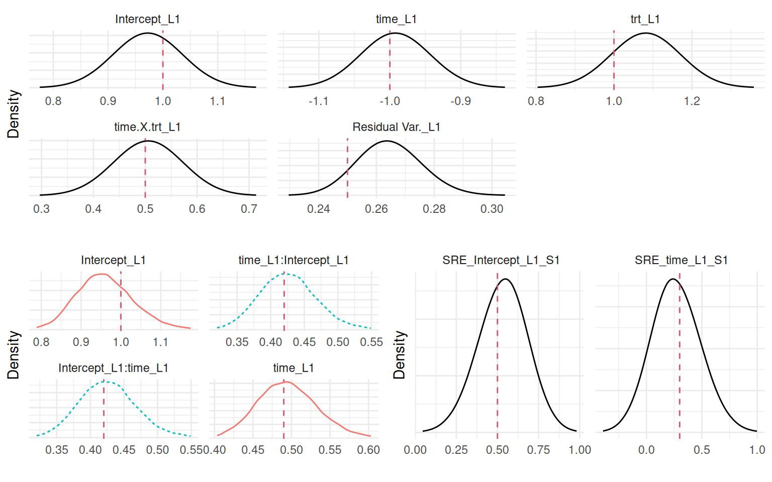
Figure 4.1 shows that the model recovered all the true parameter values. The most important ones being the association parameters since they correspond to the scaling parameters that link both submodels. As introduced in Section 1.5.3, we can see the summary of each individual random effect’s posterior distribution in the argument summary.random of the fitted object. We can compare the true values with estimates (Figure 4.2):
par(mfrow=c(1,2), mar = c(4,4,2,0.3), cex=0.8)
plot(MVnorm[,1], M_jm$summary.random$IDIntercept_L1$mean[1:n],
     xlab="True", ylab="Estimated", main="Random intercept")
plot(MVnorm[,2], M_jm$summary.random$IDtime_L1$mean[-(1:n)],
     xlab="True", ylab="Estimated", main="Random slope")
As we can see, the model did recover the individual random effects properly. This model can be used to predict the longitudinal and survival outcomes for new individuals. Let’s consider two individuals with random effects values defined as quantiles of the distribution of random effects (we consider 10% and 90% quantiles for the two individuals, so they have very different individual profiles):
SD_m <- summary(M_jm, sdcor=TRUE)$ReffList[[1]][,"mean"][1:2] # sd
SD_0 <- qnorm(p = 0.1, sd = SD_m[1]) # quantile 0.1 random intercept
SD_1 <- qnorm(p = 0.1, sd = SD_m[2]) # quantile 0.1 random slope
Y_id1 <- rnorm(6, b_0 + SD_0 + (b_1 + SD_1)*mestime, b_e) # observed id 1
Y_id2 <- rnorm(6, b_0 - SD_0 + (b_1 - SD_1)*mestime, b_e) # observed id 2
NewData <- data.frame(id=rep(1:2, each=length(mestime)),
                      time=mestime, Y=c(Y_id1, Y_id2), trt=0);NewData
id time Y trt
1 1 0 0.3421689 0
2 1 1 -1.7594623 0
3 1 2 -4.2267953 0
4 1 3 -5.3135691 0
5 1 4 -7.9560552 0
6 1 5 -10.5819121 0
7 2 0 1.9690854 0
8 2 1 3.2042589 0
9 2 2 2.3057939 0
10 2 3 1.5305130 0
11 2 4 2.0125609 0
12 2 5 0.7823775 0Now we can predict for these two individuals their individual longitudinal trajectory as well as their survival probabilities (see Section 1.5.5 for an introduction to survival curves with INLAjoint):
P <- predict(M_jm, NewData, horizon=10, survival=TRUE)
str(P)
List of 2
$ PredL:'data.frame': 102 obs. of 8 variables:
..$ id : Factor w/ 2 levels "1","2": 1 1 1 1 1 1 1 1 1 1 ...
..$ time : num [1:102] 0 0.204 0.408 0.612 0.816 ...
..$ Outcome : chr [1:102] "Y" "Y" "Y" "Y" ...
..$ Mean : num [1:102] 0.242 -0.181 -0.603 -1.026 -1.448 ...
..$ Sd : num [1:102] 0.329 0.315 0.303 0.293 0.284 ...
..$ quant0.025: num [1:102] -0.393 -0.788 -1.19 -1.596 -2.005 ...
..$ quant0.5 : num [1:102] 0.243 -0.18 -0.602 -1.025 -1.447 ...
..$ quant0.975: num [1:102] 0.89055 0.44006 -0.00585 -0.45421 -0.89437 ...
$ PredS:'data.frame': 102 obs. of 13 variables:
..$ id : Factor w/ 2 levels "1","2": 1 1 1 1 1 1 1 1 1 1 ...
..$ time : num [1:102] 0 0.204 0.408 0.612 0.816 ...
..$ Outcome : chr [1:102] "S_1" "S_1" "S_1" "S_1" ...
..$ Haz_Mean : num [1:102] 0 0 0 0 0 0 0 0 0 0 ...
..$ Haz_Sd : num [1:102] 0 0 0 0 0 0 0 0 0 0 ...
..$ Haz_quant0.025 : num [1:102] 0 0 0 0 0 0 0 0 0 0 ...
..$ Haz_quant0.5 : num [1:102] 0 0 0 0 0 0 0 0 0 0 ...
..$ Haz_quant0.975 : num [1:102] 0 0 0 0 0 0 0 0 0 0 ...
..$ Surv_Mean : num [1:102] 1 1 1 1 1 1 1 1 1 1 ...
..$ Surv_Sd : num [1:102] 1 1 1 1 1 1 1 1 1 1 ...
..$ Surv_quant0.025: num [1:102] 1 1 1 1 1 1 1 1 1 1 ...
..$ Surv_quant0.5 : num [1:102] 1 1 1 1 1 1 1 1 1 1 ...
..$ Surv_quant0.975: num [1:102] 1 1 1 1 1 1 1 1 1 1 ...Here the object P contains a list with the predictions for the longitudinal outcome PredL and the predictions for the survival outcome PredS. Both have been introduced in Section 1.5.5, and thus we do not give additional details here.
An important point to note here is that we predict the processes at future times, where we have not observed any data (all data is observed within 5 units of time and we predict at 10). In most situations, these predictions are tricky since we did not observe data and thus have to rely on the model predictions that could be far from reality. With our random walk baseline, the baseline hazard is based on the data and therefore it is not straightforward to predict in areas where no data have been observed., In this context, INLAjoint assume linear baseline hazard beyond the last observed data point. In this specific example, this choice is fine since we did simulate with constant baseline but in other situations, it may not be appropriate and predictions should be done in areas where the model did learn from the data or other baseline hazard options should be considered, such as parametric options or other proper spline models.
We can plot the estimated longitudinal trajectories, where the observed data points are displayed as black dots:
ggplot(P$PredL, aes(x = time, y = quant0.5)) + geom_line() +
  geom_ribbon(aes(ymin=quant0.025, ymax=quant0.975), alpha=0.1) +
  geom_point(data=NewData, aes(x=time, y=Y)) + ylab("Y") +
  theme(legend.position="none") + facet_wrap(~id)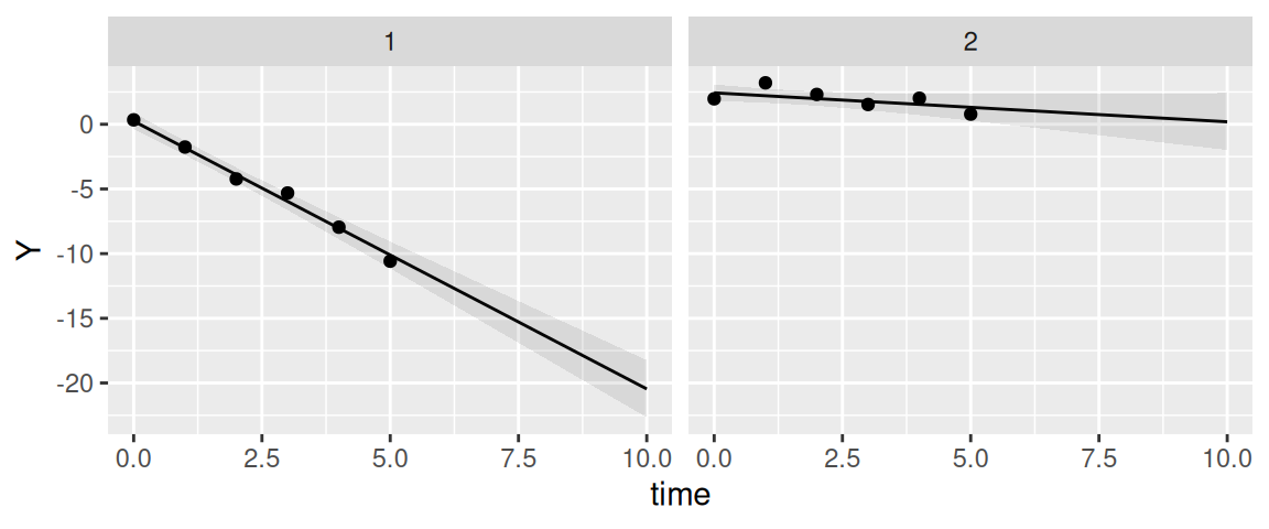
The corresponding survival probability over time is shown in Figure 4.4:
tps <- seq(5,10,len=1e3)
datTrue <- data.frame(id=rep(1:2, each=1e3), time=rep(tps,2), trt=0)
ggplot(P$PredS, aes(x = time, y = Surv_quant0.5)) + geom_line() +
 geom_ribbon(aes(ymin=Surv_quant0.025, ymax=Surv_quant0.975), alpha=0.1) +
 theme(legend.position="none") + ylab("Survival probability") +
  facet_wrap(~id)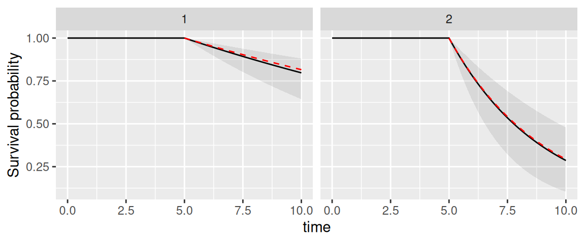
We can see that INLAjoint automatically assumes the individual was not at risk for the event until the last longitudinal measurement. This is a common assumption since in most cases the event can be recorded when assessing longitudinal measurement, and therefore when the individual produces longitudinal measurements it also means the individual is event-free at this time. In some situations, we may consider the individual is at risk at a specific time, which can be defined with the argument Csurv. For example we can consider our 2 individuals were at risk since time 0:
P <- predict(M_jm, NewData, horizon=10, survival=TRUE, Csurv=0)
tps <- seq(5,10,len=1e3)
ggplot(P$PredS, aes(x = time, y = Surv_quant0.5)) + geom_line() +
 geom_ribbon(aes(ymin=Surv_quant0.025, ymax=Surv_quant0.975), alpha=0.1) +
 theme(legend.position="none") + facet_wrap(~id)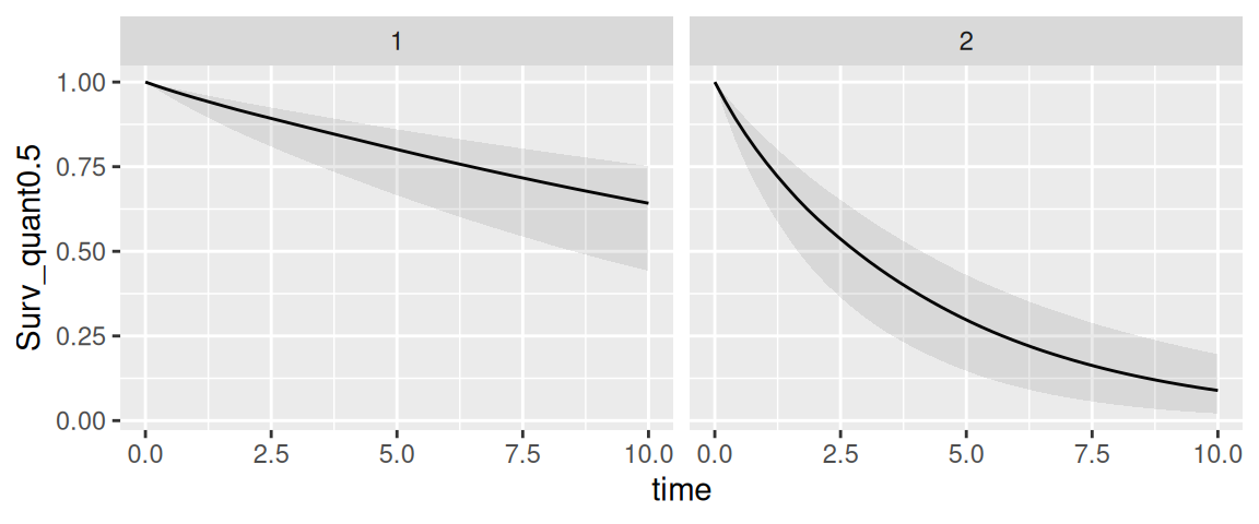
4.3.2 Time-dependent individual deviation from the average longitudinal trajectory
Building upon the shared random effects association structure, a more sophisticated approach involves incorporating a time-dependent component into the survival submodel. In this association structure, the survival model includes a linear combination of the random effects from the longitudinal model. This accounts for the dynamic nature of the relationship between the longitudinal measurements and the survival outcomes, where the event risk depends on the individual deviation from the population average of the longitudinal marker trajectory.
The purpose of this time-dependent association structure is to capture the relationship between the evolving longitudinal and survival processes. By allowing the shared component to change over time, the model can better reflect the reality that an individual’s risk of an event may vary as their longitudinal trajectory changes. While this structure introduces additional complexity compared to the previous shared random effects association, it can lead to more accurate predictions and inference. The model is defined as follows: \[\begin{equation*}
\left\{ \begin{array}{lc}
\textrm{E}[Y_{i}(t)]= \beta_0 + b_{i0} + (\beta_1 + b_{i1})\cdot t + \beta_2\cdot trt_i + \beta_3\cdot trt_i\cdot t \\
\lambda_i(t)=\lambda_0(t)\exp\left(\gamma\cdot \left(b_{i0} + b_{i1}\cdot t\right)\right)
\end{array}
\right.
\end{equation*}\] Simulating an event time becomes more complex when the hazard function itself includes a time-dependent component. Unlike the shared random effects model in the previous section where the term in the exponent was constant over time for a given individual, here it changes linearly with time \(t\). This means the hazard rate is not constant, even with an exponential baseline. To generate an event time using the inverse transform sampling method, we must first compute the cumulative hazard function \(\Lambda_i(t)=\int_0^t \lambda_i(s)\mathrm{d}s\), needed for the computation of survival. When the linear predictor includes time-dependent components, there is often no closed-form analytical solution for the integral over the risk. This challenge requires the use of specialized numerical algorithms to generate event times from a complex, time-varying hazard function. These methods typically work by discretizing the follow-up time into a fine grid of small intervals. Within each interval, the time-dependent covariate (and thus the hazard) can be treated as approximately constant, allowing for the step-wise calculation of the cumulative hazard. An event time is then generated based on this numerically approximated survival function. The R package PermAlgo uses a permutation algorithm to generate event times conditional on time-dependent covariates by performing a one-to-one matching of subjects to a set of pre-generated event times based on a probability law derived from the Cox partial likelihood. Of note, permAlgo cannot provide the true baseline hazard because its core permutation algorithm is specifically designed to generate survival data without ever needing to specify or compute a baseline hazard function.
gap2 <- 0.01 # used to generate a lot of time points for PermAlgo
mestime2 <- seq(0,fw,gap2) # measurement times
time2 <- rep(mestime2, n) # time column
n_i2 <- length(mestime2)
trt2 <- rep(trt, each=n_i2)
b12 <- rep(MVnorm[,1], each=n_i2)
b22 <- rep(MVnorm[,2], each=n_i2)
SRE_i <- b12 + b22*time2 # linear combination of random effects to share
# Permutation algorithm to generate survival times that depends on SRE_i
library(PermAlgo)
DatTmp <- permalgorithm(n, n_i2, Xmat=matrix(SRE_i, ncol=1), betas=s_1)
DatTmp2 <- DatTmp[which(!duplicated(DatTmp$Id, fromLast = T)),
                  c("Id","Event","Stop")]
datJM2_S <- data.frame(id = 1:n, eventTimes = mestime2[DatTmp2$Stop+1],
                       eventIndic = DatTmp2$Event, trt = trt)
datJM2_L <- datJM_Lt[-unlist(sapply(1:n, function(x)
  which(datJM_Lt$time>=datJM2_S$eventTimes[datJM2_S$id==x] &
          datJM_Lt$id==x))),]
Now we have our two datasets with the desired structure. We can fit the joint model, the call of the joint() function is the same as the previous model except for the association parameter assoc="SRE" which stands for “shared random effects” (i.e., sharing the individual deviation from the mean at time t as defined by the random effects).
M_jmSRE <- joint(formSurv = inla.surv(eventTimes, eventIndic) ~ -1,
                 formLong = Y ~ time * trt + (1 + time | id),
                 dataSurv = datJM2_S, dataLong=datJM2_L,
                 id="id", timeVar="time", assoc="SRE")
The data structure is different from the previous model because now we need to account for the time-dependent association. With R-INLA, this is done by including an additional layer in the data to compute the linear combination of parameters to share.
str(M_jmSRE$.args$data)List of 24
$ Intercept_L1 : num [1:6878] 1 1 1 1 1 1 1 1 1 1 ...
$ time_L1 : num [1:6878] 0 1 0 1 0 1 0 1 2 0 ...
$ trt_L1 : num [1:6878] 1 1 0 0 1 1 1 1 1 1 ...
$ time.X.trt_L1 : num [1:6878] 0 1 0 0 0 1 0 1 2 0 ...
$ IDIntercept_L1 : num [1:6878] 1 1 2 2 3 3 4 4 4 5 ...
$ IDtime_L1 : num [1:6878] 501 501 502 502 503 503 504 504 504 505 ...
$ WIntercept_L1 : num [1:6878] 1 1 1 1 1 1 1 1 1 1 ...
$ Wtime_L1 : num [1:6878] 0 1 0 1 0 1 0 1 2 0 ...
$ usre1 : num [1:6878] NA NA NA NA NA NA NA NA NA NA ...
$ wsre1 : num [1:6878] NA NA NA NA NA NA NA NA NA NA ...
$ Y_L1 : num [1:6878] 1.865 1.824 -0.196 -2.188 2.295 ...
$ SRE_L1_S11 : num [1:6878] NA NA NA NA NA NA NA NA NA NA ...
$ y1..coxph : num [1:6878] NA NA NA NA NA NA NA NA NA NA ...
$ E..coxph : num [1:6878] NA NA NA NA NA NA NA NA NA NA ...
$ expand1..coxph : int [1:6878] NA NA NA NA NA NA NA NA NA NA ...
$ baseline1.hazard : num [1:6878] NA NA NA NA NA NA NA NA NA NA ...
$ baseline1.hazard.idx : num [1:6878] NA NA NA NA NA NA NA NA NA NA ...
$ baseline1.hazard.time : num [1:6878] NA NA NA NA NA NA NA NA NA NA ...
$ baseline1.hazard.length: num [1:6878] NA NA NA NA NA NA NA NA NA NA ...
$ Intercept_S1 : num [1:6878] NA NA NA NA NA NA NA NA NA NA ...
$ SRE_L1_S1 : num [1:6878] NA NA NA NA NA NA NA NA NA NA ...
$ id : int [1:6878] NA NA NA NA NA NA NA NA NA NA ...
$ baseline1.hazard.values: num [1:16] 0 0.325 0.651 0.976 1.301 ...
$ Yjoint :List of 3
..$ Y_L1 : num [1:6878] 1.865 1.824 -0.196 -2.188 2.295 ...
..$ SRE_L1_S11: num [1:6878] NA NA NA NA NA NA NA NA NA NA ...
..$ y1..coxph : num [1:6878] NA NA NA NA NA NA NA NA NA NA ...We can see the outcome now is a list of 3 outcomes where the second one is there to compute the linear combination of parameters to share from the longitudinal to the survival model. We can have a look at the data structure for the first individual, starting with the longitudinal components:
id1 <- which(M_jmSRE$.args$data$IDIntercept_L1==1 | M_jmSRE$.args$data$expand1..coxph==1)
sapply(M_jmSRE$.args$data[c(1:6,8,11)], function(x) round(x[id1], 2))
Intercept_L1 time_L1 trt_L1 time.X.trt_L1 IDIntercept_L1 IDtime_L1 Wtime_L1 Y_L1
[1,] 1 0 1 0 1 501 0.00 1.86
[2,] 1 1 1 1 1 501 1.00 1.82
[3,] NA NA NA NA 1 501 0.16 NA
[4,] NA NA NA NA 1 501 0.49 NA
[5,] NA NA NA NA 1 501 0.81 NA
[6,] NA NA NA NA 1 501 1.14 NA
[7,] NA NA NA NA NA NA NA NA
[8,] NA NA NA NA NA NA NA NA
[9,] NA NA NA NA NA NA NA NA
[10,] NA NA NA NA NA NA NA NAWe can see that the first 2 lines correspond to the longitudinal submodel while the next 4 lines are used to compute the linear combination of random effects, these lines only includes the id of the random effects and the weight of the random slope (note that the weight corresponds to the middle of the corresponding survival interval where the linear combination of parameters is shared), other fixed effects are not shared and thus set to NA on these lines. We can also have a look at the survival part:
sapply(M_jmSRE$.args$data[c(14,16,8,9,21,13)], function(x) round(x[id1], 2)) E..coxph baseline1.hazard Wtime_L1 usre1 SRE_L1_S1 y1..coxph
[1,] NA NA 0.00 NA NA NA
[2,] NA NA 1.00 NA NA NA
[3,] NA NA 0.16 1 NA NA
[4,] NA NA 0.49 2 NA NA
[5,] NA NA 0.81 3 NA NA
[6,] NA NA 1.14 4 NA NA
[7,] 0.33 0.00 NA NA 1 0
[8,] 0.33 0.33 NA NA 2 0
[9,] 0.33 0.65 NA NA 3 0
[10,] 0.21 0.98 NA NA 4 1The column usre1 and SRE_L1_S1 are used to link the linear combination of parameters to share and the survival part. For example we can see from line 3 that the linear combination of the random effects is computed at time ~0.16, which is the middle of the first interval of the survival submodel which starts at time 0 and ends at time 0.33 (line 7). We therefore assume this interval is associated to the linear combination of the random effects computed at the middle of the interval (more intervals then leads to a more detailed representation of the longitudinal marker in the survival process). The formula to fit this model is also more involved with R-INLA, since we need to indicate that we want to compute the linear combination of random effects, which is done as follows:
cat(attr(terms(M_jmSRE$.args$formula), which = "term.labels")[9])f(usre1, wsre1, model = "iid", hyper = list(prec = list(initial = -6, fixed = TRUE)), constr = F)This is required to create a specific outcome (with value 0) that acts as “fake” Gaussian observations where the linear combination of parameters is computed at specified time points. Then we need to indicate that we want to share this linear combination of parameters in the survival submodel:
cat(attr(terms(M_jmSRE$.args$formula), which = "term.labels")[10])f(SRE_L1_S1, copy = "usre1", hyper = list(beta = list(fixed = FALSE, param = c(0, 0.01), initial = 0.1)))Of note, when functions of time are included in the longitudinal model, it is important to provide the function as presented in Section 3.2.5 because the shared part needs to be computed at many time points internally (i.e., the value of the shared component is computed at the middle of each time interval for each individual) to properly account for its evolution over time in the risk function.
We can have a look at the summary of our model fitted with INLAjoint:
summary(M_jmSRE, sdcor=TRUE)Longitudinal outcome (gaussian)
mean sd 0.025quant 0.5quant 0.975quant
Intercept_L1 0.9895 0.0647 0.8626 0.9895 1.1166
time_L1 -1.0640 0.0581 -1.1773 -1.0642 -0.9495
trt_L1 1.0311 0.0901 0.8543 1.0311 1.2078
time:trt_L1 0.4990 0.0739 0.3540 0.4990 0.6440
Res. err. (sd) 0.5161 0.0205 0.4779 0.5153 0.5585
Random effects standard deviation / correlation (L1)
mean sd 0.025quant 0.5quant 0.975quant
Intercept_L1 0.9898 0.0407 0.9155 0.9871 1.0757
time_L1 0.6865 0.0397 0.6117 0.6847 0.7690
Intercept_L1:time_L1 0.5590 0.0673 0.4183 0.5626 0.6807
Survival outcome
mean sd 0.025quant 0.5quant 0.975quant
Baseline risk (variance)_S1 0.7106 0.1485 0.4697 0.693 1.0517
Association longitudinal - survival
mean sd 0.025quant 0.5quant 0.975quant
SRE_L1_S1 0.4728 0.0419 0.3916 0.4723 0.5566
log marginal-likelihood (integration) log marginal-likelihood (Gaussian)
-14039.36 -14035.34
Deviance Information Criterion: 4366.229
Widely applicable Bayesian information criterion: 4328.681
Computation time: 5.57 secondsIn this model, the association is defined by a single coefficient, SRE_L1_S1, which quantifies the association between the subject’s current deviation from the population-average trajectory and his risk of event. This structure is different compared to Section 4.3.1 as it assumes that the deviation from the mean trajectory, rather than its separate components (intercept and slope), is what drives the risk.
This means that the impact of an individual’s latent characteristics on their risk of event changes over time. For example, consider an individual with a high positive random intercept (\(b_{i0} > 0\)) but a strong negative random slope (\(b_{i1}\) < 0). At early time points, his deviation from the mean is positive, leading to an increased hazard (assuming \(\gamma=\) 0.47). However, as time progresses, his trajectory crosses below the population average, and the term (\(b_{0i}+b_{1i}t\)) becomes negative, leading to a decreased hazard compared to population average. This structure allows the model to capture how an individual’s risk profile evolves as his biomarker deviates from the average over the follow-up.
We can plot the posterior marginals of all parameters as shown in Figure 4.6:
Plots_jm <- plot(M_jmSRE)
ggarrange(eval(parse(text=P1)),
          ggarrange(eval(parse(text=P2)),
                    eval(parse(text=P3)), ncol=2), nrow=2)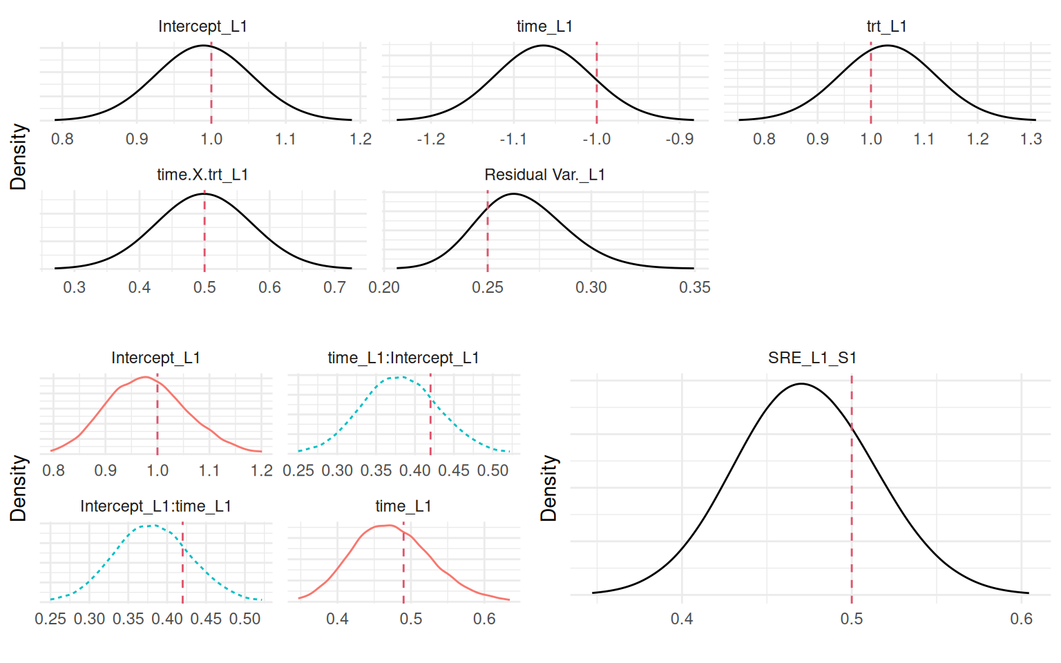
We can see that the model is able to recover the true values of all the parameters. Since we simulated event times with a permutation algorithm, the true baseline hazard function is assumed unknown and the default random walk is used. We can also predict from this model, let’s for example consider the first two individuals of the dataset used to fit the model and predict at horizon 5:
NewData <- datJM2_L[datJM2_L$id %in% 1:2,]
P <- predict(M_jmSRE, NewData, horizon=5, survival=TRUE)
P_1 <- ggplot(P$PredL, aes(x = time, y = quant0.5)) + geom_line() +
  geom_ribbon(aes(ymin=quant0.025, ymax=quant0.975), alpha=0.1) +
  geom_point(data=NewData, aes(x=time, y=Y)) + ylab("Y") +
  theme(legend.position="none") + facet_wrap(~id)
P_2 <- ggplot(P$PredS, aes(x = time, y = Surv_quant0.5)) + geom_line() +
  geom_ribbon(aes(ymin=Surv_quant0.025, ymax=Surv_quant0.975),alpha=0.1) +
  theme(legend.position="none") + ylab("Survival probability") +
  facet_wrap(~id)
ggarrange(P_1,P_2, nrow=2)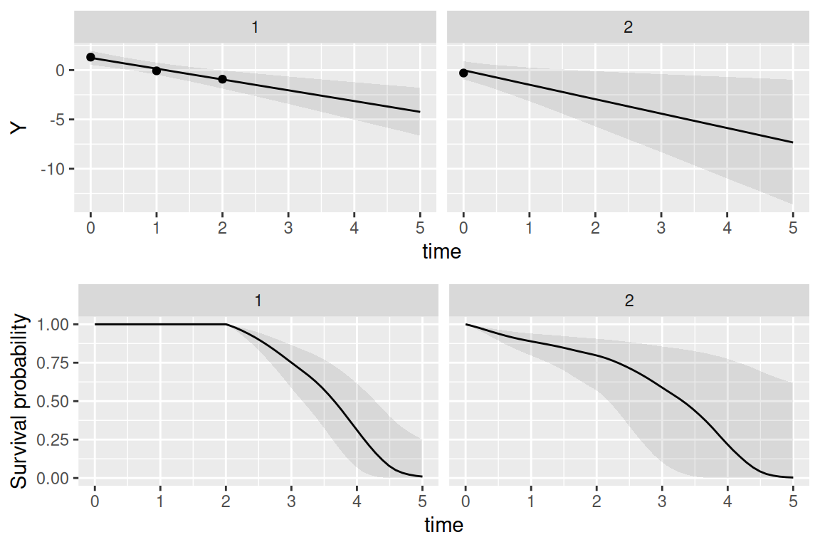
We can see how the uncertainty of the prediction for both outcomes depends on the amount of data provided.
4.3.3 Current value association structure
The current value association structure is similar to the previous one but fixed effects are shared in addition to the random effects, such that the risk of the event depends on the expected value of the linear predictor from the longitudinal submodel, sometimes refered to as the “true” value of the marker since it does not include the residual error (which could be noise coming from the tools that produce the measurement for example). The model is defined as follows: \[\begin{equation*} \left\{ \begin{array}{rl} \textrm{E}[Y_{i}(t)]&= \eta_i(t)\\ &= \beta_0 + b_{i0} + (\beta_1 + b_{i1})\cdot t + \beta_2\cdot trt_i + \beta_3\cdot trt_i\cdot t\\ \lambda_i(t)&=\lambda_0(t)\exp\left(\gamma \cdot \eta_i(t)\right) \end{array} \right. \end{equation*}\] Where the risk of event \(\lambda\) for individual \(i\) at time \(t\) depends on the linear predictor \(\eta\) for individual \(i\) at time \(t\) through the scaling parameter \(\gamma\). The association parameter is interpreted as the log-hazard ratio for a one-unit increase in this true biomarker value. Unlike the SRE structure, the CV structure incorporates the influence of all covariates (e.g., treatment) on the longitudinal marker directly into the risk of event calculation.
We can simulate data from this model with the same strategy as for the previous section, where we first compute the time-dependent component to share (here, the linear predictor without the noise), an we can generate survival times using the permutation algorithm.
CV_i <- b_0 + b12 + (b_1 + b22)*time2 + b_2*trt2 + b_3*trt2*time2
DatTmp <- permalgorithm(n, n_i2, Xmat=matrix(CV_i, ncol=1), betas=c(s_1))
DatTmp2 <- DatTmp[which(!duplicated(DatTmp$Id, fromLast = T)),
                  c("Id","Event","Stop")]
datJM3_S <- data.frame(id = 1:n, eventTimes = mestime2[DatTmp2$Stop+1],
                       eventIndic = DatTmp2$Event, trt = trt)
datJM3_L <- datJM_Lt[-unlist(sapply(1:n, function(x)
  which(datJM_Lt$time>=datJM3_S$eventTimes[datJM3_S$id==x] &
          datJM_Lt$id==x))),]
And we can fit the model with the following call, where the association parameter is assoc="CV", which stands for “current value” (of the linear predictor, sometimes referred to as “current level”):
M_jmCV <- joint(formSurv = inla.surv(eventTimes, eventIndic) ~ -1,
                formLong = Y ~ time * trt + (1 + time | id),
                dataSurv = datJM3_S, dataLong=datJM3_L,
                id="id", timeVar="time", assoc="CV")
summary(M_jmCV, sdcor=TRUE)
Longitudinal outcome (gaussian)
mean sd 0.025quant 0.5quant 0.975quant
Intercept_L1 0.9637 0.0674 0.8315 0.9636 1.0959
time_L1 -0.9974 0.0610 -1.1162 -0.9977 -0.8767
trt_L1 1.1156 0.0983 0.9227 1.1156 1.3084
time:trt_L1 0.4466 0.0936 0.2632 0.4466 0.6306
Res. err. (sd) 0.5294 0.0210 0.4899 0.5287 0.5724
Random effects standard deviation / correlation (L1)
mean sd 0.025quant 0.5quant 0.975quant
Intercept_L1 0.9778 0.0418 0.8974 0.9774 1.0590
time_L1 0.6877 0.0390 0.6167 0.6872 0.7675
Intercept_L1:time_L1 0.5992 0.0672 0.4564 0.6035 0.7132
Survival outcome
mean sd 0.025quant 0.5quant 0.975quant
Baseline risk (variance)_S1 0.7714 0.1377 0.5402 0.7578 1.0803
Association longitudinal - survival
mean sd 0.025quant 0.5quant 0.975quant
CV_L1_S1 0.492 0.0429 0.4083 0.4918 0.5771
log marginal-likelihood (integration) log marginal-likelihood (Gaussian)
-13745.92 -13741.90
Deviance Information Criterion: 4227.396
Widely applicable Bayesian information criterion: 4189.455
Computation time: 5.73 secondsNow the association is CV_L1_S1 for the effect of the current value of the first longitudinal submodel effect on the risk of the first survival outcome. We can plot the posterior marginals:
Plots_jm <- plot(M_jmCV)
ggarrange(eval(parse(text=P1)),
          ggarrange(eval(parse(text=P2)),
                    eval(parse(text=P3)), ncol=2), nrow=2)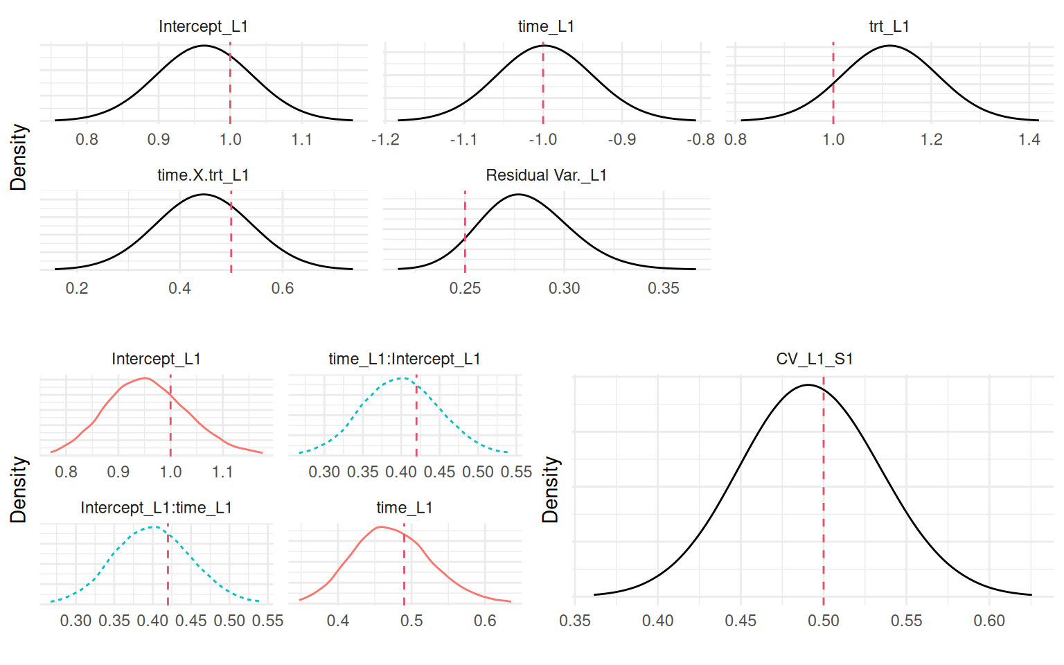
Of note, the current value (CV) and shared random effects (SRE) associations are equivalent in the absence of covariates in the longitudinal part of the model and when the covariates are also included in the survival part, because in these cases the hazard is simply shifted by a constant.
4.3.4 Current slope association structure
While the previous association assume that the risk of event at time \(t\) depends on the value of the outcome at the same time \(t\), we may be more interested in the dynamic behavior of the marker. The derivative of the linear predictor with respect to time, describes some aspect of the evolution of the marker. It corresponds to the trend (or the rate of change) at time \(t\), where a positive value means the marker is increasing while a negative means it decreases. It is sometimes of interest to assume that the risk of event depends on the trend of the marker at time \(t\), rather than its value. The association parameter is then the log-hazard ratio for a one-unit increase in this rate of change. Accounting for the current slope of the biomarker provides a different perspective on the risk, allowing the model to distinguish between individuals who may have the same marker level but different underlying trends.
For instance, if two patients have a biomarker value of 10, but one’s marker is rapidly increasing while the other’s is decreasing, the CS structure can estimate if the former has a higher risk, independent of their current value. We can define the following model: \[\begin{equation*} \left\{ \begin{array}{rl} \textrm{E}[Y_{i}(t)]&= \eta_i(t)\\ &= \beta_0 + b_{i0} + (\beta_1 + b_{i1})\cdot t + \beta_2\cdot trt_i + \beta_3\cdot trt_i\cdot t \\ \lambda_i(t)&=\lambda_0(t)\exp\left(\gamma\cdot \left(\frac{\mathrm{d}\eta_i(t)}{\mathrm{d}t}\right)\right) \end{array} \right. \end{equation*}\] Where the derivative of the linear predictor from the longitudinal submodel is shared and scaled with parameter \(\gamma\). Given the simplicity of the proposed model, our derivative only includes the fixed effect of time, the random slope as well as the treatment effect over time.
For more complex longitudinal models, such as described in Section 3.2.5, where splines are used to describe the evolution of the marker over time, the current slope parametrization in INLAjoint is computing the derivative of the linear predictor numerically using the R package NumDeriv (Gilbert & Varadhan (2019)), which requires to setup any function of time as described in Section 3.2.5. We can simulate data from the same random intercept-slope model as in previous sections:
CS_i <- (b_1 + b22) + b_3*trt2
DatTmp <- permalgorithm(n, n_i2, Xmat=matrix(CS_i, ncol=1), betas=c(s_1))
DatTmp2 <- DatTmp[which(!duplicated(DatTmp$Id, fromLast = T)),
                  c("Id","Event","Stop")]
datJM4_S <- data.frame(id = 1:n, eventTimes = mestime2[DatTmp2$Stop+1],
                       eventIndic = DatTmp2$Event, trt = trt)
datJM4_L <- datJM_Lt[-unlist(sapply(1:n, function(x)
  which(datJM_Lt$time>=datJM4_S$eventTimes[datJM4_S$id==x] &
          datJM_Lt$id==x))),]
And we can fit the model by simply setting the argument assoc="CS", which stands for “current slope” (of the linear predictor):
M_jmCS <- joint(formSurv = inla.surv(eventTimes, eventIndic) ~ -1,
                formLong = Y ~ time * trt + (1 + time | id),
                dataSurv = datJM4_S, dataLong=datJM4_L,
                id="id", timeVar="time", assoc="CS")
Internally the data has the same structure as with assoc="CV", except that now only fixed and random effects that interacts with time or functions of time are contributing to the shared part. We can directly plot the posterior marginals to compare with true values used for data generation:
Plots_jm <- plot(M_jmCS)
ggarrange(eval(parse(text=P1)),
          ggarrange(eval(parse(text=P2)),
                    eval(parse(text=P3)), ncol=2), nrow=2)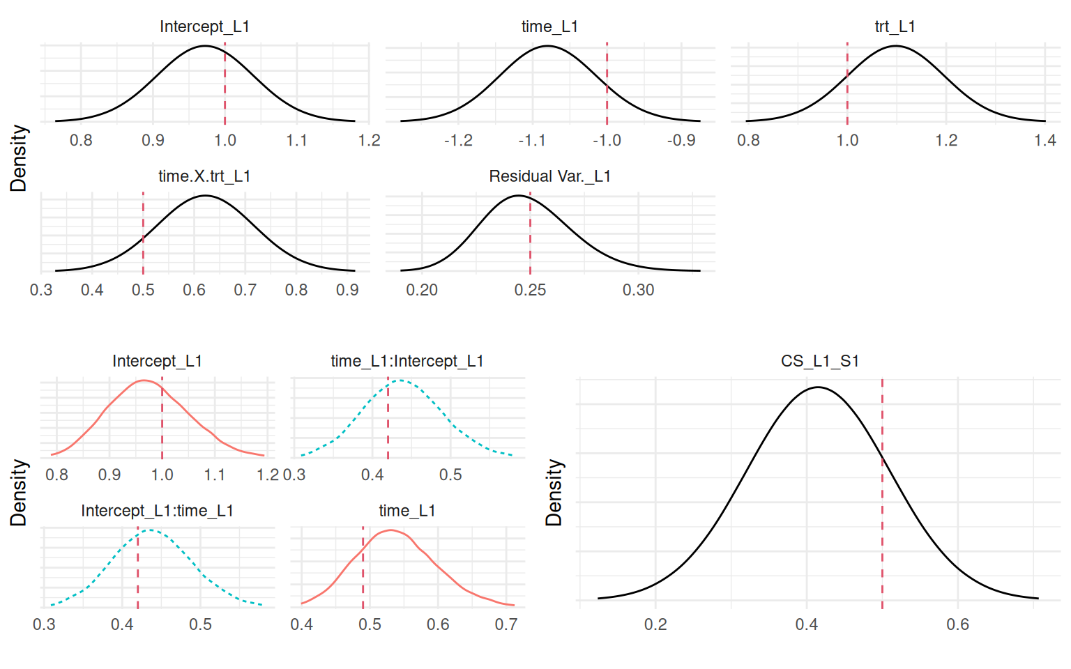
Again, the model is able to capture all the parameters posterior from the data information.
4.3.5 Current value and current slope association structure
We may be interested in both the effect of the value of the marker as well as its rate of change on the risk of an event. This can be done with the association assoc="CV_CS", which simply combines the two previous options. The corresponding model is: \[\begin{equation*}
\left\{ \begin{array}{rl}
\textrm{E}[Y_{i}(t)]&= \eta_i(t)\\
&= \beta_0 + b_{i0} + (\beta_1 + b_{i1})\cdot t + \beta_2\cdot trt_i + \beta_3\cdot trt_i\cdot t \\
\lambda_i(t)&=\lambda_0(t)\exp\left(\gamma_1\cdot \eta_i(t) + \gamma_2\cdot \left(\frac{\mathrm{d}\eta_i(t)}{\mathrm{d}t}\right)\right)
\end{array}
\right.
\end{equation*}\] This model includes two association parameters allowing for the simultaneous evaluation of both the marker’s level and its trend effect on the risk of event. This model can evaluate if a high biomarker value is increasing the risk in itself and whether an increase in the biomarker confers an additional risk, even after accounting for its current value. This structure is useful when both the state and the dynamics of a disease process are thought to be prognostic. We can simulate data from this model using the permutation algorithm, where the event times are conditional on two time-dependent components:
DatTmp <- permalgorithm(n, n_i2,
                        Xmat=matrix(c(CV_i, CS_i), ncol=2),
                        betas=c(s_1, s_2)) # association
DatTmp2 <- DatTmp[which(!duplicated(DatTmp$Id, fromLast = T)),
                  c("Id","Event","Stop")]
datJM5_S <- data.frame(id = 1:n, eventTimes = mestime2[DatTmp2$Stop+1],
                       eventIndic = DatTmp2$Event, trt = trt)
datJM5_L <- datJM_Lt[-unlist(sapply(1:n, function(x)
  which(datJM_Lt$time>=datJM5_S$eventTimes[datJM5_S$id==x] &
          datJM_Lt$id==x))),]
Then we can fit the model:
M_jmCVCS <- joint(formSurv = inla.surv(eventTimes, eventIndic) ~ -1,
                  formLong = Y ~ time * trt + (1 + time | id),
                  dataSurv = datJM5_S, dataLong=datJM5_L,
                  id="id", timeVar="time", assoc="CV_CS")
and we can have a look at the results:
Plots_jm <- plot(M_jmCVCS)
ggarrange(eval(parse(text=P1)),
          ggarrange(eval(parse(text=P2)),
                    eval(parse(text=P3)), ncol=2), nrow=2)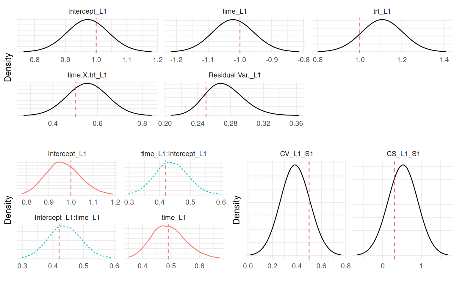
4.3.6 Cumulative value with area under the curve association structure
So far we assumed associations where the hazard at time \(t\) depends on components from the longitudinal marker at time \(t\). For some applications, this does not sound appropriate, for example let’s consider the relationship between air pollution and the risk of lung cancer. The risk at time \(t\) could be explained by some accumulated exposure up to \(t\) but may not be related to the exposure at \(t\). In such context, we are interested in the cumulative effect of the marker on the risk of event at time \(t\). By integrating the longitudinal trajectory over time, this association structure captures the overall exposure to the longitudinal marker. Unlike simpler association structures that rely on current values or random effects, this approach considers the entire history of the longitudinal measurements up to a given time point. The cumulative value association structure is implemented by including the integral of the longitudinal trajectory as a time-dependent covariate in the survival submodel. Because of the decomposition of the follow-up in small intervals, we can compute the required integral directly with a linear combination of the parameters.
When sharing the current value of the linear predictor (see Section 4.3.3), the linear predictor of the longitudinal is computed for each interval of the follow-up of the survival, such that the weight of the shared component is a diagonal identity matrix (i.e., each computed value of the linear predictor corresponds to one interval of the survival submodel). We can take advantage of this structure and change this diagonal identity matrix to weight the linear predictor such that each interval of follow-up includes the linear predictor of previous intervals.
The model is defined as follows: \[\begin{equation*} \left\{ \begin{array}{rl} \textrm{E}[Y_{i}(t)]&= \eta_i(t)\\ &= \beta_0 + b_{i0} + (\beta_1 + b_{i1})\cdot t + \beta_2\cdot trt_i + \beta_3\cdot trt_i\cdot t \\ \lambda_i(t)&=\lambda_0(t)\exp\left(\gamma \cdot \int_{s=0}^{t}\eta_i(s)\mathcal{d}s\right) \end{array} \right. \end{equation*}\] We define the interval to start at time 0 here, such that the entire history of the marker affects the risk at time \(t\) but we could also assume a specific window of exposure, as illustrated hereafter.
Let’s start by simulating some data. First we compute cumulative values of the marker, reusing the linear predictor simulated earlier for simplicity. Then we use the permutation algorithm to simulate event times that depend on the time-dependent area under the curve of the biomarker.
CUM_CV_i <- rep(NA, length(CV_i))
for(i in 1:n){
  CUM_CV_i[(n_i2*(i-1)+1):((n_i2*i))] <- cumsum(
    c(0, CV_i[(n_i2*(i-1)+1):((n_i2*i)-1)])*gap2)
}
DatTmp <- permalgorithm(n, n_i2, Xmat=matrix(CUM_CV_i, ncol=1), betas=s_1)
DatTmp2 <- DatTmp[which(!duplicated(DatTmp$Id, fromLast = T)),
                  c("Id","Event","Stop")]
datJM6_S <- data.frame(id = 1:n, eventTimes = mestime2[DatTmp2$Stop+1],
                       eventIndic = DatTmp2$Event, trt = trt)
datJM6_L <- datJM_Lt[-unlist(sapply(1:n, function(x)
  which(datJM_Lt$time>=datJM6_S$eventTimes[datJM6_S$id==x] &
          datJM_Lt$id==x))),]
Here, the risk at time \(t\) depends on the cumulative value of the marker since time \(0\). We start by defining the joint model with current value association structure, but we do not run the INLA algorithm yet by adding the argument run=FALSE (see Section 1.5.8):
M_jmCUM_CV0 <- joint(formSurv = inla.surv(eventTimes, eventIndic) ~ -1,
                formLong = Y ~ time * trt + (1 + time | id),
                dataSurv = datJM6_S, dataLong=datJM6_L,
                id="id", timeVar="time", assoc="CV",
                run=FALSE)
Now we want to replace the weights for the shared current value, we first need to create a matrix of weights. We can extract from the object we just created the size of each follow-up interval in the survival part of the joint model:
w <- na.omit(M_jmCUM_CV0$.args$data$E..coxph);head(w)[1] 0.33 0.33 0.28 0.33 0.33 0.33Here the length of an interval is 0.33 but some intervals are smaller when an event or right censoring is observed. The corresponding id of each follow-up interval can also be extracted:
w.idx <- na.omit(M_jmCUM_CV0$.args$data$baseline1.hazard.idx);head(w.idx)[1] 1 2 3 1 2 3We can see that first 3 intervals are for first individual, which was right censored after 0.33+0.33+0.28=0.94 units of time:
datJM6_S[1,] id eventTimes eventIndic trt
1 1 0.94 0 1Based on the extracted information, we can create a matrix to compute the cumulative value of the marker over the follow-up for each individual at each time point. For each follow-up interval included, we scale the value by the size of the interval (of note, the value of the linear predictor computed for the current value association structure is computed for the middle of the time interval).
w.size <- length(M_jmCUM_CV0$.args$data$baseline1.hazard.values)
maxSize <- w.size==length(M_jmCUM_CV0$.args$data$baseline1.hazard.values)
nA <- length(w)
nT <- length(M_jmCUM_CV0$.args$data$Intercept_L1)
j.acc <- 0
ijx <- list(i = rep(0L, w.size * nA),
            j = rep(0L, w.size * nA),
            x = rep(0.0, w.size * nA))
nacc = 0;
for(i in 1:nA) {
  iw <- tail(1:w.idx[i], w.size)
  ni <- length(iw)
  if((i>1) & (w.idx[i]==1)) j.acc <- j.acc + w.idx[i-1]
  jj <- j.acc + iw
  w0 <- w[jj]
  fixw <- (!maxSize & tail(w0, 1)<(0.99*w0[1]))
  if((length(jj)>1) && fixw) {
    iw <- tail(1:w.idx[i], w.size+1)
    ni <- length(iw)
    jj <- j.acc + iw
    w0 <- w[jj]
    w0[1] <- w0[1]-tail(w0,1)
  }
  ijx$i[nacc + 1:ni] <- i
  ijx$j[nacc + 1:ni] <- jj
  ijx$x[nacc + 1:ni] <- w0
  nacc <- nacc + ni
}
A0 <- sparseMatrix(i = ijx$i[1:nacc],
                   j = ijx$j[1:nacc],
                   x = ijx$x[1:nacc])
Adata <- rbind(sparseMatrix(i=1, j=1, x=0, dims = c((nT-nA), nA)), A0)
inla.as.sparse(A0[1:10,1:10])
10 x 10 sparse Matrix of class "dgTMatrix"
[1,] 0.33 . . . . . . . . .
[2,] 0.33 0.33 . . . . . . . .
[3,] 0.33 0.33 0.28 . . . . . . .
[4,] . . . 0.33 . . . . . .
[5,] . . . 0.33 0.33 . . . . .
[6,] . . . 0.33 0.33 0.33 . . . .
[7,] . . . 0.33 0.33 0.33 0.33 . . .
[8,] . . . 0.33 0.33 0.33 0.33 0.19 . .
[9,] . . . . . . . . 0.33 .
[10,] . . . . . . . . 0.33 0.33We can see the upper-left of the weight matrix we have created. The first line corresponds to the first follow-up interval for the first individual, it scales the value of the marker by the length of this interval (0.33). The third line is the third (and last) follow-up interval for individual 1. It includes the cumulative value of the marker over the first, second and third interval with a lower weight for the last interval because this individual was censored before the end of the interval. Now we can include this weight matrix in the data and the formula of the object we created before running the INLA algorithm. We use the option A.local in the f() call to scale the current value with a matrix:
M_jmCUM_CV0$.args$data$WCUM <- rep(0, nT)
M_jmCUM_CV0$.args$formula <- as.formula(paste(c("Yjoint ~ -1 ",
   attr(terms(M_jmCUM_CV0$.args$formula), which = "term.labels")[1:9],
   "+ f(CV_L1_S1, WCUM, copy = 'uv1', hyper = list(beta = list(
   fixed = FALSE, param = c(0, 0.01), initial = 0.1)),
   A.local = Adata)"), collapse="+"))
M_jmCUM_CV <- joint.run(M_jmCUM_CV0)
Here we defined the prior for the association parameter firectly in the f() call, within the R-INLA environment, where param = c(0, 0.01) corresponds to a Gaussian prior with mean 0 and variance 100 and initial = 0.1 is the initial value. This is the same prior as the default prior for other time-dependent associations in INLAjoint, which is usually a reasonable choice.
Now we have fitted the model, where “CV_L1_S1” corresponds to the cumulative exposure effect on the risk of event, we can display the posterior marginals and compare with true values:
Plots_jm <- plot(M_jmCUM_CV)
ggarrange(eval(parse(text=P1)),
          ggarrange(eval(parse(text=P2)),
                    eval(parse(text=P3)), ncol=2), nrow=2)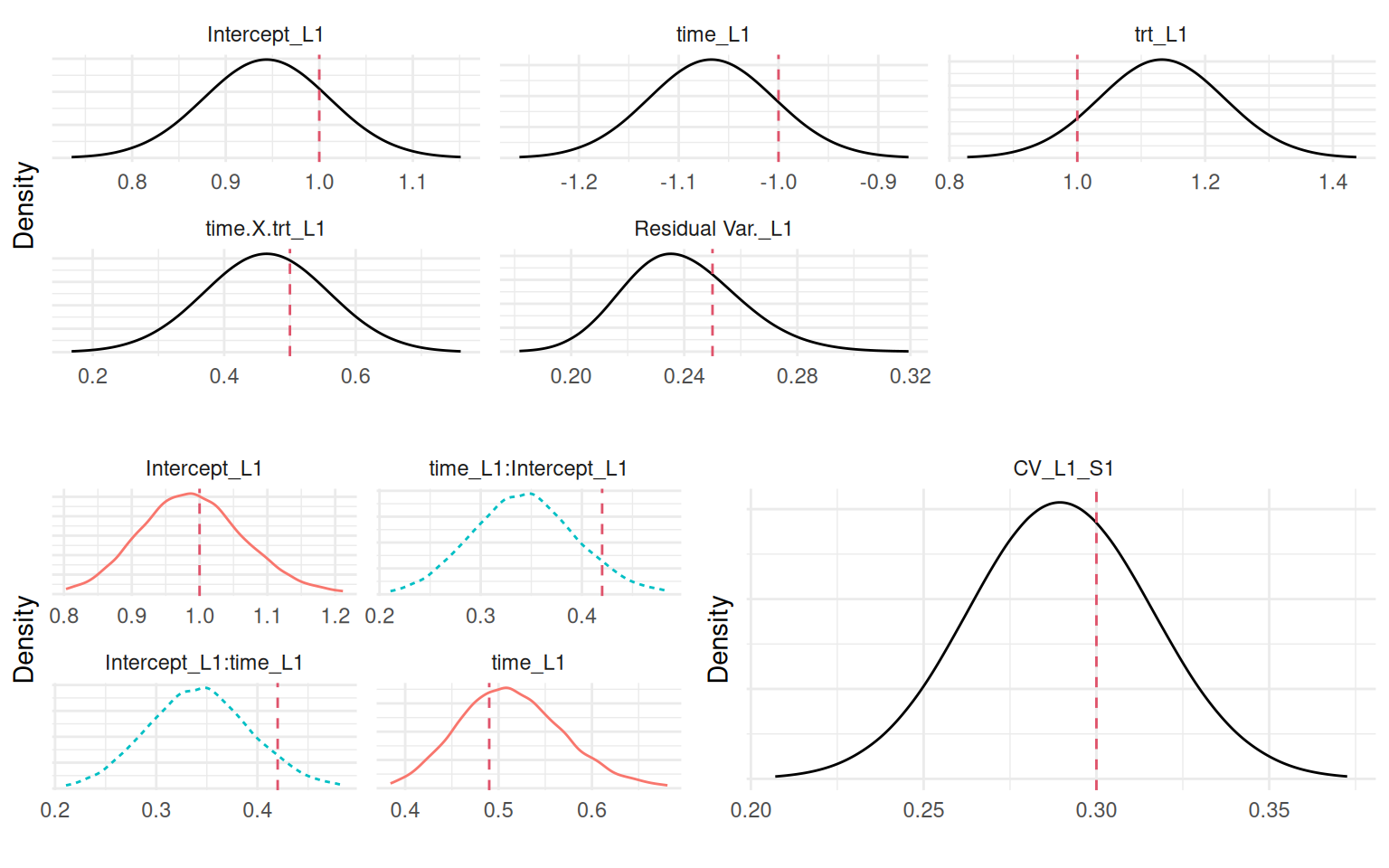
We assumed the cumulative exposure is computed since time 0 for each individual. We may instead consider that we want the risk at time \(t\) to depend only on a specific window in the past, rather than the entire history of the longitudinal marker. Here we kept the default interval size which is 0.33, of course we could get a finer resolution by increasing the number of intervals with the argument NbasRisk as described in Chapter 2. If we want the risk at time t to depend on the last 2 intervals (i.e., up to 0.66 units of time in the past), we can adjust the matrix with weights as follows:
10 x 10 sparse Matrix of class "dgTMatrix"

 [1,] 0.33 .    .    .    .    .    .    .    .    .
 [2,] 0.33 0.33 .    .    .    .    .    .    .    .
 [3,] 0.05 0.33 0.28 .    .    .    .    .    .    .
 [4,] .    .    .    0.33 .    .    .    .    .    .
 [5,] .    .    .    0.33 0.33 .    .    .    .    .
 [6,] .    .    .    .    0.33 0.33 .    .    .    .
 [7,] .    .    .    .    .    0.33 0.33 .    .    .
 [8,] .    .    .    .    .    0.14 0.33 0.19 .    .
 [9,] .    .    .    .    .    .    .    .    0.33 .
[10,] .    .    .    .    .    .    .    .    0.33 0.33
We can see in this matrix that only 0.66 units of time in the past are included, such that the risk for an individual at time \(t\) depends on the cumulative exposure of the last 0.66 units of time. It is easy to see how changing this matrix can adjust the computation of the association structure. One can also see how this approach allows to consider lagged effect, for any association structure presented before.
4.3.7 Non-linear association structure
The association structures presented so far, such as the shared random effects (SRE), current value (CV) and current slope (CS), involves a unique, constant parameter \(\gamma\) scaling each shared component from longitudinal submodels in survival submodels. \[\begin{equation*} \begin{array}{rl} \lambda_i(t)&=\lambda_0(t)\exp\left(\gamma \cdot h(\cdot)\right) \end{array} \end{equation*}\] Here, \(h(\cdot)\) represents a shared component derived from the longitudinal submodel, such as the current value of the linear predictor or its derivative. This formulation assume a linear relationship between the shared component and the log-risk of an event, providing a straightforward and interpretable framework. However, this linear assumption, while convenient, may be overly restrictive in real-world scenarios where the true effect of the shared component on the survival outcome is more complex.
In many clinical and epidemiological contexts, the risk profile may follow a non-monotonic pattern. For instance, consider the association between Body Mass Index (BMI) and all-cause mortality. A linear association would incorrectly imply that each unit increase in BMI is associated to a constant change in mortality risk. The well-established reality, however, is a U-shaped curve: both very low (underweight) and very high (obese) BMI values are associated with an increased mortality risk compared to an healthy, intermediate range. In such cases, a linear association structure could be misleading. The positive risk effects at the two extremes of the BMI distribution would cancel each other out, leading to erroneously conclude that no association exists when, in fact, a strong and clinically meaningful non-linear relationship is present.
This section introduces a hierarchical framework to define non-linear association structures, offering greater flexibility by allowing the effect of the shared component to vary depending on its value. Let’s consider the contribution of the shared component to the log-hazard with the standard association: \[\begin{equation*} \begin{array}{rl} \log(HR)&=\gamma \cdot h(\eta_i(t)) \end{array} \end{equation*}\] This equation shows that the log-hazard is a linear function of the shared component \(h(\eta_i(t))\). This is similar to a simple linear regression model, \(y=\beta_0+\beta_1x\), where the parameter \(\beta_1\) is a constant that defines a linear relationship between x and y. In the context of the joint model, a one-unit increase in the shared component is associated with a constant change of \(\gamma\) in the log-hazard, regardless of the value of the component. Therefore, we can refer to this standard structure as a “linear association on the log-hazard scale” or “constant scaling effect”.
To move beyond the linear assumption, we can generalize the association structure by replacing the constant scaling parameter \(\gamma\) with a function, \(f(\cdot)\), that depends on the value of the shared component itself. The generalized hazard function then becomes: \[\begin{equation*} \begin{array}{rl} \lambda_i(t)&=\lambda_0(t)\exp\left(f(h(\eta_i(t))) \cdot h(\eta_i(t))\right) \end{array} \end{equation*}\] In this formulation, the term \(f(h(\eta_i(t)))\) can be interpreted as a value-dependent scaling parameter. The model is then transformed from having a single scalar \(\gamma\), to a function \(f(\cdot)\). We propose a hierarchical set of models that correspond to different parametrizations of this scaling function, each offering an additional layer of flexibility.
The first extension of the standard model allows the scaling effect to vary linearly with the value of the shared component. This is achieved by defining the scaling function \(f(⋅)\) as a simple linear function: \[f(x)=\gamma_1+\gamma_2\cdot x\] where \(x=h(\eta_i(t))\). The resulting contribution to the log-hazard is now a quadratic function of the shared component: \[\begin{equation*} \begin{array}{rl} \log(HR)&=\gamma_1\cdot h(\eta_i(t)) + \gamma_2\cdot h(\eta_i(t))^2 \end{array} \end{equation*}\] This model allows the effect of the shared component to change depending on its value. The parameter \(\gamma_1\) can be interpreted as a linear effect on the log-hazard while \(\gamma_2\) captures a quadratic effect. This structure is capable of modeling simple non-monotonic relationships, making it suitable for capturing U-shaped or inverted U-shaped associations.
An important point here is that this model can reduce to the standard linear association model. If the posterior distribution for the curvature parameter \(\gamma_2\) is concentrated around zero, the model reduces to the standard form with a constant scaling effect of \(\gamma_1\). This provides a natural, data-driven path for model simplification and comparison.
While the quadratic association offers more flexibility than the linear form, it is still constrained to a parabolic shape. To capture more complex relationships, we can generalize the scaling function by adding a non-parametric smooth term. This is achieved using a second-order random walk (RW2), a form of Bayesian smooth spline.
The scaling function is then defined as: \[f(x)=\gamma_1+\gamma_2\cdot x + \textrm{RW2}(x)\] The full hazard model becomes: \[\begin{equation*} \begin{array}{rl} \lambda_i(t)&=\lambda_0(t)\exp\left((\gamma_1 + \gamma_2\cdot h(\eta_i(t)) + \textrm{RW2}(h(\eta_i(t)))) \cdot h(\eta_i(t))\right) \end{array} \end{equation*}\] The component \(\textrm{RW2}(\cdot)\) represents a flexible, zero-mean deviation from the underlying linear trend defined by \(\gamma_1\) and \(\gamma_2\). This is the same type of random walk model used to flexibly model the baseline hazard (Section 2.2.3). The RW2 is a Gaussian process that penalizes the second differences of its components, which encourages smoothness by penalizing sharp changes in the slope of the function. The RW2 component is defined by a precision parameter that controls its degree of smoothness. The prior placed on this precision parameter, typically a penalized complexity prior (Section 1.1.2.1), is constructed to shrink the non-linear component towards zero unless there is sufficient evidence in the data to support a more complex function.
In practice, this model is implemented by discretizing the observed range of the shared component into a set of knots. The RW2 is then defined over these knots, and its value for any given \(h(\eta_i(t))\) is determined by interpolation. The number of knots, which controls the maximum potential flexibility, can be specified by the user (via the n_NL argument), though a small number (e.g., 3-5) is often sufficient for most applications.
This structure allows the model to adapt its complexity based on the information available in the data. Moreover, model selection can be performed by fitting separate models for each level of complexity (linear, quadratic, and spline) and comparing them using goodness-of-fit criteria such as the Deviance Information Criterion (DIC) or the Widely Applicable Bayesian Information Criterion (WAIC), which are directly available in the INLAjoint output (see Section 1.5.3).
The hierarchical Bayesian formulation offers an integrated approach. If the true relationship is quadratic, the posterior distribution for the RW2 variance will be concentrated near zero, causing the model to collapse to the quadratic association. If the true relationship is a simple linear association on the log-hazard scale, the posterior for the RW2 variance and the posterior for \(\gamma_2\) will both be concentrated near zero, causing the model to collapse further to the standard association.
We can illustrate the differences in terms of raw effect (\(f(h(\eta_i(t)))\)), log-hazard ratios (\(f(h(\eta_i(t)))\cdot h(\eta_i(t))\)) and the corresponding hazard ratios (\(\exp\left(f(h(\eta_i(t)))\cdot h(\eta_i(t))\right)\)) as follows:
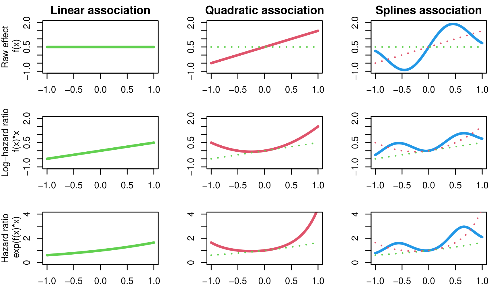
We can see how each level of complexity is adding flexibility built upon the previous model.
Let’s consider the model fitted in Section 4.3.2, with a standard current value association, in order to fit the model with a linear effect, the association argument has to be modified to add “L_” (for “Linear”), such that the parameter is now assoc="L_CV":
M_jmLCV <- joint(formSurv = inla.surv(eventTimes, eventIndic) ~ -1,
                 formLong = Y ~ time * trt + (1 + time | id),
                 dataSurv = datJM3_S, dataLong=datJM3_L,
                 id="id", timeVar="time", assoc="L_CV")
summary(M_jmLCV, sdcor=TRUE)
Longitudinal outcome (gaussian)
mean sd 0.025quant 0.5quant 0.975quant
Intercept_L1 0.9639 0.0674 0.8318 0.9639 1.0961
time_L1 -0.9964 0.0610 -1.1153 -0.9968 -0.8757
trt_L1 1.1151 0.0983 0.9223 1.1151 1.3078
time:trt_L1 0.4477 0.0936 0.2643 0.4477 0.6317
Res. err. (sd) 0.5300 0.0210 0.4905 0.5294 0.5732
Random effects standard deviation / correlation (L1)
mean sd 0.025quant 0.5quant 0.975quant
Intercept_L1 0.9761 0.0392 0.9030 0.9747 1.0583
time_L1 0.6875 0.0394 0.6140 0.6868 0.7653
Intercept_L1:time_L1 0.5989 0.0678 0.4541 0.6047 0.7177
Survival outcome
mean sd 0.025quant 0.5quant 0.975quant
Baseline risk (variance)_S1 0.7724 0.1292 0.55 0.7618 1.057
Association longitudinal - survival
mean sd 0.025quant 0.5quant 0.975quant
Beta0 for NL_CV_L1_S1 0.4838 0.0396 0.4064 0.4835 0.5624
Beta1 for NL_CV_L1_S1 0.0676 0.1082 -0.1521 0.0698 0.2736
log marginal-likelihood (integration) log marginal-likelihood (Gaussian)
-37224.29 -37219.34
Deviance Information Criterion: 4227.757
Widely applicable Bayesian information criterion: 4190.427
Computation time: 10 secondsWe can see the summary has now two parameters, Beta0 for the intercept (\(\gamma_1\)) and Beta1 for the slope (\(\gamma_2\)). We can see the intercept with a value close to the true value (0.5) and a slope almost equal to zero (because the true model has a constant effect of 0.5).
Non-linear associations can be plotted with the plot function. The default call will plot the scaled effect (i.e., the log-hazard ratio \(f(x)*x\)). It is possible to plot only the raw effect by adding the argument NLeffectonly=TRUE in the call of the plot function. It is also possible to get the hazard ratio when hr=TRUE is included in the call of the plot function:
Pl1 <- plot(M_jmLCV)$NL_Association
Pl1$data$Effect <- "Log hazard ratio"
Pl2 <- plot(M_jmLCV, NLeffectonly=T)$NL_Associations
Pl2$data$Effect <- "Raw effect"
Pl3 <- plot(M_jmLCV, hr=T)$NL_Associations
Pl3$data$Effect <- "Hazard ratio"
ggarrange(Pl2, Pl1, Pl3, nrow=1)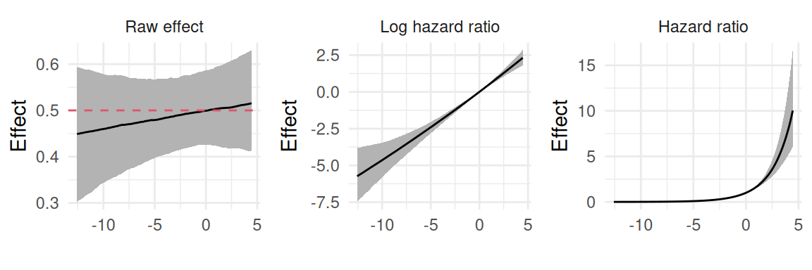
Here the x axis is the shared component value (i.e., the value of the shared linear predictor that corresponds to the expected value of the longitudinal marker in this case). We can see the the raw effect is roughly constant and includes the true value (0.5). We can have a look at goodness of fit criteria which both show a roughly similar fit between the two models, meaning that adding a slope here does not make a big difference.
GOF <- data.frame("Linear" = c(M_jmCV$dic$dic, M_jmCV$waic$waic),
                  "Quadratic" = c(M_jmLCV$dic$dic, M_jmLCV$waic$waic))
rownames(GOF) <- c("DIC", "WAIC");GOF
Linear Quadratic
DIC 4227.396 4227.757
WAIC 4189.455 4190.427Now let’s consider an example where there is non-linearity in the effect. For example we can have the following true model: \[\begin{equation*} \left\{ \begin{array}{rl} \textrm{E}[Y_{i}(t)]&= \eta_i(t)\\ &= \beta_0 + b_{i0} + \beta_1\cdot t + \beta_2\cdot trt_i + \beta_3\cdot trt_i\cdot t \\ \lambda_i(t)&=\lambda_0(t)\exp\left(\eta_i(t) \cdot\frac{\eta_i(t)}{30}\right) \end{array} \right. \end{equation*}\] Here the effect of the current value has a “U” shape. We can start by simulating data from this model, reusing the linear predictor simulated in Section 4.3.3:
# NL function
F_NL <- function(x) x*x/30
NLCV_i <- F_NL(CV_i) # non-linear effect's full contribution to log HR
DatTmp <- permalgorithm(n, n_i2, Xmat=matrix(NLCV_i, ncol=1), betas=1)
DatTmp2 <- DatTmp[which(!duplicated(DatTmp$Id, fromLast = T)),
                  c("Id","Event","Stop")]
datJM7_S <- data.frame(id = 1:n, eventTimes = mestime2[DatTmp2$Stop+1],
                       eventIndic = DatTmp2$Event, trt = trt)
datJM7_L <- datJM_Lt[-unlist(sapply(1:n, function(x)
  which(datJM_Lt$time>=datJM7_S$eventTimes[datJM7_S$id==x] &
          datJM_Lt$id==x))),]
Now we can fit the models with each level of flexibility and compare their estimated association. We start by fitting the model with linear and quadratic associations:
M_jmCV2 <- joint(formSurv = inla.surv(eventTimes, eventIndic) ~ -1,
                 formLong = Y ~ time * trt + (1 + time | id),
                 dataSurv = datJM7_S, dataLong=datJM7_L,
                 id="id", timeVar="time", assoc="CV")
summary(M_jmCV2)
Longitudinal outcome (gaussian)
mean sd 0.025quant 0.5quant 0.975quant
Intercept_L1 0.9775 0.0669 0.8464 0.9775 1.1086
time_L1 -1.0372 0.0646 -1.1644 -1.0371 -0.9109
trt_L1 1.0891 0.0973 0.8983 1.0891 1.2799
time:trt_L1 0.4515 0.0946 0.2664 0.4513 0.6377
Res. err. (variance) 0.2796 0.0231 0.2376 0.2784 0.3282
Random effects variance-covariance (L1)
mean sd 0.025quant 0.5quant 0.975quant
Intercept_L1 0.9294 0.0800 0.7799 0.9256 1.0968
time_L1 0.5090 0.0576 0.4050 0.5051 0.6281
Intercept_L1:time_L1 0.4310 0.0544 0.3234 0.4303 0.5393
Survival outcome
mean sd 0.025quant 0.5quant 0.975quant
Baseline risk (variance)_S1 0.0868 0.0694 0.021 0.0658 0.279
Association longitudinal - survival
mean sd 0.025quant 0.5quant 0.975quant
CV_L1_S1 -0.0663 0.0323 -0.13 -0.0663 -0.0028
log marginal-likelihood (integration) log marginal-likelihood (Gaussian)
-13817.87 -13813.93
Deviance Information Criterion: 4408.996
Widely applicable Bayesian information criterion: 4369.813
Computation time: 4.01 secondsM_jmLCV2 <- joint(formSurv = inla.surv(eventTimes, eventIndic) ~ -1,
formLong = Y ~ time * trt + (1 + time | id),
dataSurv = datJM7_S, dataLong=datJM7_L,
id="id", timeVar="time", assoc="L_CV")
summary(M_jmLCV2)Longitudinal outcome (gaussian)
mean sd 0.025quant 0.5quant 0.975quant
Intercept_L1 0.9773 0.0669 0.8461 0.9773 1.1084
time_L1 -1.0342 0.0648 -1.1618 -1.0341 -0.9074
trt_L1 1.0896 0.0973 0.8987 1.0895 1.2805
time:trt_L1 0.4638 0.0952 0.2777 0.4636 0.6512
Res. err. (variance) 0.2771 0.0229 0.2357 0.2759 0.3257
Random effects variance-covariance (L1)
mean sd 0.025quant 0.5quant 0.975quant
Intercept_L1 0.9343 0.0777 0.7907 0.9323 1.0927
time_L1 0.5163 0.0593 0.4102 0.5137 0.6391
Intercept_L1:time_L1 0.4380 0.0538 0.3298 0.4358 0.5471
Survival outcome
mean sd 0.025quant 0.5quant 0.975quant
Baseline risk (variance)_S1 0.1174 0.0799 0.027 0.0968 0.3312
Association longitudinal - survival
mean sd 0.025quant 0.5quant 0.975quant
Beta0 for NL_CV_L1_S1 -0.0611 0.0264 -0.1132 -0.0611 -0.0090
Beta1 for NL_CV_L1_S1 0.3814 0.0941 0.1922 0.3828 0.5628
log marginal-likelihood (integration) log marginal-likelihood (Gaussian)
-37289.54 -37284.46
Deviance Information Criterion: 4386.447
Widely applicable Bayesian information criterion: 4342.622
Computation time: 8.3 secondsThe model with spline association, which is the most flexible level, can be fitted by including “NL_” in the assoc argument as follows:
M_jmNLCV2 <- joint(formSurv = inla.surv(eventTimes, eventIndic) ~ -1,
                   formLong = Y ~ time * trt + (1 + time | id),
                   dataSurv = datJM7_S, dataLong=datJM7_L,
                   id="id", timeVar="time", assoc="NL_CV")
summary(M_jmNLCV2)
Longitudinal outcome (gaussian)
mean sd 0.025quant 0.5quant 0.975quant
Intercept_L1 0.9779 0.0668 0.8469 0.9779 1.1090
time_L1 -1.0380 0.0650 -1.1659 -1.0379 -0.9109
trt_L1 1.0890 0.0972 0.8983 1.0890 1.2797
time:trt_L1 0.4640 0.0952 0.2778 0.4638 0.6514
Res. err. (variance) 0.2735 0.0207 0.2370 0.2719 0.3183
Random effects variance-covariance (L1)
mean sd 0.025quant 0.5quant 0.975quant
Intercept_L1 0.9432 0.0781 0.8015 0.9392 1.1066
time_L1 0.5213 0.0580 0.4160 0.5178 0.6463
Intercept_L1:time_L1 0.4373 0.0483 0.3438 0.4366 0.5399
Survival outcome
mean sd 0.025quant 0.5quant 0.975quant
Baseline risk (variance)_S1 0.0828 0.0333 0.0459 0.0736 0.1723
Association longitudinal - survival
mean sd 0.025quant 0.5quant 0.975quant
Beta0 for NL_CV_L1_S1 -0.0560 0.0292 -0.1121 -0.0564 0.0027
Beta1 for NL_CV_L1_S1 0.4265 0.1143 0.2267 0.4197 0.6731
Beta2 for NL_CV_L1_S1 0.0208 0.0361 -0.0466 0.0196 0.0954
Beta3 for NL_CV_L1_S1 -0.0388 0.0588 -0.1645 -0.0356 0.0654
Beta4 for NL_CV_L1_S1 0.0188 0.0598 -0.0904 0.0162 0.1443
log marginal-likelihood (integration) log marginal-likelihood (Gaussian)
-37295.19 -37288.43
Deviance Information Criterion: 4385.667
Widely applicable Bayesian information criterion: 4336.351
Computation time: 10.48 secondsNow we have 5 parameters for the association in this last model, the first two are still the intercept and slope but now we have 3 parameters associated to the random walk that allows deviations from the linear effect. The number of knots for the spline part (i.e., random walk of order 2) can be chosen in the control options with argument n_NL. In most situations, the default 3 knots should be sufficient and adding more knots only allows to capture very complex non-linear effects that are uncommon in real world data. We can plot the hazard ratios obtained with the 3 models:
Assoc_value <- summary(M_jmCV2, sdcor=TRUE, hr=T)$AssocLS[,c(1,3,5)]
Pl1 <- plot(M_jmLCV2, hr=T)$NL_Associations
Pl2 <- plot(M_jmNLCV2, hr=T)$NL_Associations
par(mar = c(4,4,2,0.3))
plot(datJM7_L$Y, exp(F_NL(datJM7_L$Y)), cex=0.7,
     xlim=c(range(datJM7_L$Y)), ylim=c(0.9,4), xlab="Current value",
     ylab="Hazard ratio", pch=16)
abline(h=Assoc_value[1], lwd=3, col=2, lty=3)
abline(h=Assoc_value[2], col=2, lty=3)
abline(h=Assoc_value[3], col=2, lty=3)
lines(Pl1$data$x, Pl1$data$y, lwd=3, col=3)
lines(Pl1$data$x, Pl1$data$lower, col=3)
lines(Pl1$data$x, Pl1$data$upper, col=3)
lines(Pl2$data$x, Pl2$data$y, lwd=3, col=4, lty=2)
lines(Pl2$data$x, Pl2$data$lower, col=4, lty=2)
lines(Pl2$data$x, Pl2$data$upper, col=4, lty=2)
legend(x = -3, y = 4, c("True", "Linear", "Quadratic", "Spline"),
       col=1:4, lty=c(0,3,1,2), lwd=3, pch=c(16,NA,NA,NA), seg.len = 3)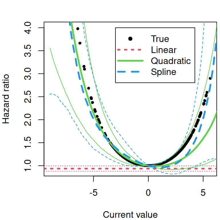
Here we clearly see that the linear association cannot capture this non-linear curve while the other two approaches are able to get the true association The standard joint model even concludes to no association because the increased risk for low values of the marker are canceled by the increased risk for higher values. We also notice that adding more flexibility with the spline association does not seem necessary here since the model with a quadratic effect performs well, it results in slightly more uncertainty.
Interpreting this plot requires moving beyond a fixed hazard ratio to a dynamic risk profile that is conditional on an individual’s latent traits, such as the time-dependent current value of the biomarker. While the U-shaped curve itself is at the population level, an individual’s biomarker value defines his position along it, which can evolve as his biomarker evolves over time.
We can see a clear improvement in goodness of fit for the non-linear association models compared to the standard association:
GOF <- data.frame("Linear" = c(M_jmCV2$dic$dic, M_jmCV2$waic$waic),
                  "Quadratic" = c(M_jmLCV2$dic$dic, M_jmLCV2$waic$waic),
                  "Spline" = c(M_jmNLCV2$dic$dic, M_jmNLCV2$waic$waic))
rownames(GOF) <- c("DIC", "WAIC");GOF
Linear Quadratic Spline
DIC 4408.996 4386.447 4385.667
WAIC 4369.813 4342.622 4336.351Let’s consider an example where only the model with spline effect is expected to perform well: \[\begin{equation*} \left\{ \begin{array}{rl} \textrm{E}[Y_{i}(t)]&= \eta_i(t)\\ &= \beta_0 + b_{i0} + \beta_1\cdot t + \beta_2\cdot trt_i + \beta_3\cdot trt_i\cdot t \\ \lambda_i(t)&=\lambda_0(t)\exp\left(b_{i0} \cdot\log(b_{i0}^2+1)\right) \end{array} \right. \end{equation*}\] Here the shared component is only a random intercept, scaled by a non-linear function. We can simulate from this model:
# NL function
b1NL <- rnorm(n, sd=0.5) # random intercept longi with NL effect on surv
F_NL <- function(x) x*log(x^2+1) # NL function
linPred <- b_0 + rep(b1NL, each=n_i) + b_1*time + b_2*trtY + b_3*trtY*time
Y <- rnorm(n_i*n, linPred, b_e) # observed outcome
datJM_Lt2 <- data.frame(id, time, Y, trt=trtY)
eventTimes <- -(log(u)/(baseScale*exp(F_NL(b1NL)*1)))
eventIndic <- as.numeric(eventTimes<fw) # eventTimes indicator
## censoring individuals at end of follow-up (not at random)
eventTimes <- pmin(eventTimes, fw)
datJM8_S <- data.frame(id=1:n, eventTimes, eventIndic, trt) # survival
## removing longi measurements after death
datJM8_L <- datJM_Lt2[-unlist(sapply(1:n,
              function(x) which(datJM_Lt2$time>=
                                  datJM6_S$eventTimes[datJM6_S$id==x] &
                                  datJM_Lt2$id==x))),]
Based on this data, we can fit the models with the 3 levels of flexibility:
M_jmSRE2 <- joint(formSurv = inla.surv(eventTimes, eventIndic) ~ -1,
                 formLong = Y ~ time * trt + (1 + time | id),
                 dataSurv = datJM8_S, dataLong=datJM8_L,
                 id="id", timeVar="time", assoc="SRE")
Assoc_value <- summary(M_jmSRE2, sdcor=TRUE, hr=T)$AssocLS[,c(1,3,5)]
summary(M_jmSRE2)
Longitudinal outcome (gaussian)
mean sd 0.025quant 0.5quant 0.975quant
Intercept_L1 1.0245 0.0396 0.9468 1.0245 1.1021
time_L1 -1.0347 0.0269 -1.0875 -1.0347 -0.9820
trt_L1 0.9661 0.0581 0.8522 0.9661 1.0801
time:trt_L1 0.5037 0.0442 0.4170 0.5037 0.5903
Res. err. (variance) 0.2321 0.0150 0.2041 0.2316 0.2631
Random effects variance-covariance (L1)
mean sd 0.025quant 0.5quant 0.975quant
Intercept_L1 0.2245 0.0284 0.1767 0.2222 0.2869
time_L1 0.0339 0.0066 0.0230 0.0332 0.0482
Intercept_L1:time_L1 -0.0241 0.0123 -0.0506 -0.0234 -0.0025
Survival outcome
mean sd 0.025quant 0.5quant 0.975quant
Baseline risk (variance)_S1 0.0182 0.0266 3e-04 0.009 0.0925
Association longitudinal - survival
mean sd 0.025quant 0.5quant 0.975quant
SRE_L1_S1 0.2322 0.2095 -0.1783 0.2315 0.6465
log marginal-likelihood (integration) log marginal-likelihood (Gaussian)
-25558.91 -25555.04
Deviance Information Criterion: 3855.775
Widely applicable Bayesian information criterion: 3857.632
Computation time: 6.46 secondsM_jmLSRE2 <- joint(formSurv = inla.surv(eventTimes, eventIndic) ~ -1,
formLong = Y ~ time * trt + (1 + time | id),
dataSurv = datJM8_S, dataLong=datJM8_L,
id="id", timeVar="time", assoc="L_SRE")
Pl1 <- plot(M_jmLSRE2, hr=T)$NL_Associations
summary(M_jmLSRE2)Longitudinal outcome (gaussian)
mean sd 0.025quant 0.5quant 0.975quant
Intercept_L1 1.0239 0.0395 0.9464 1.0239 1.1015
time_L1 -1.0347 0.0269 -1.0875 -1.0347 -0.9819
trt_L1 0.9669 0.0579 0.8533 0.9669 1.0806
time:trt_L1 0.5041 0.0442 0.4174 0.5041 0.5908
Res. err. (variance) 0.2328 0.0151 0.2045 0.2323 0.2639
Random effects variance-covariance (L1)
mean sd 0.025quant 0.5quant 0.975quant
Intercept_L1 0.2281 0.0307 0.1758 0.2250 0.2989
time_L1 0.0343 0.0068 0.0232 0.0336 0.0495
Intercept_L1:time_L1 -0.0273 0.0137 -0.0606 -0.0260 -0.0045
Survival outcome
mean sd 0.025quant 0.5quant 0.975quant
Baseline risk (variance)_S1 0.0142 0.0197 2e-04 0.0072 0.0696
Association longitudinal - survival
mean sd 0.025quant 0.5quant 0.975quant
Beta0 for NL_SRE_L1_S1 0.2270 0.1836 -0.1316 0.2260 0.5913
Beta1 for NL_SRE_L1_S1 1.0021 0.7248 -0.4166 0.9993 2.4371
log marginal-likelihood (integration) log marginal-likelihood (Gaussian)
-75226.40 -75221.61
Deviance Information Criterion: 3857.197
Widely applicable Bayesian information criterion: 3858.323
Computation time: 17.72 secondsM_jmNLSRE2 <- joint(formSurv = inla.surv(eventTimes, eventIndic) ~ -1,
formLong = Y ~ time * trt + (1|id),
dataSurv = datJM8_S, dataLong=datJM8_L,
id="id", timeVar="time", assoc="NL_SRE")
Pl2 <- plot(M_jmNLSRE2, hr=T)$NL_Associations
summary(M_jmNLSRE2)Longitudinal outcome (gaussian)
mean sd 0.025quant 0.5quant 0.975quant
Intercept_L1 1.0235 0.0391 0.9469 1.0235 1.1001
time_L1 -1.0356 0.0214 -1.0775 -1.0356 -0.9936
trt_L1 0.9678 0.0575 0.8552 0.9678 1.0805
time:trt_L1 0.5053 0.0372 0.4325 0.5053 0.5782
Res. err. (variance) 0.2495 0.0125 0.2264 0.2490 0.2754
Random effects variance-covariance (L1)
mean sd 0.025quant 0.5quant 0.975quant
Intercept_L1 0.2028 0.0157 0.1727 0.2026 0.2345
Survival outcome
mean sd 0.025quant 0.5quant 0.975quant
Baseline risk (variance)_S1 0.0428 0.0098 0.0251 0.0425 0.0631
Association longitudinal - survival
mean sd 0.025quant 0.5quant 0.975quant
Beta0 for NL_SRE_L1_S1 0.3576 0.1163 0.1505 0.3517 0.6060
Beta1 for NL_SRE_L1_S1 0.2282 0.1949 -0.1211 0.2179 0.6423
Beta2 for NL_SRE_L1_S1 0.3889 0.0941 0.2024 0.3893 0.5729
Beta3 for NL_SRE_L1_S1 -0.0150 0.0633 -0.1471 -0.0125 0.1017
Beta4 for NL_SRE_L1_S1 0.0156 0.0629 -0.1001 0.0131 0.1469
log marginal-likelihood (integration) log marginal-likelihood (Gaussian)
-75225.84 -75218.20
Deviance Information Criterion: 3841.008
Widely applicable Bayesian information criterion: 3850.068
Computation time: 7.73 secondsAnd we can display their association:
par(mar = c(4,4,2,0.3))
plot(b1NL, exp(F_NL(b1NL)), cex=0.7,
     xlim=c(range(b1NL)), ylim=c(0,3), xlab="Random effect value",
     ylab="Hazard ratio", pch=16)
abline(h=Assoc_value[1], lwd=3, col=2, lty=3)
abline(h=Assoc_value[2], col=2, lty=3)
abline(h=Assoc_value[3], col=2, lty=3)
lines(Pl1$data$x, Pl1$data$y, lwd=3, col=3)
lines(Pl1$data$x, Pl1$data$lower, col=3)
lines(Pl1$data$x, Pl1$data$upper, col=3)
lines(Pl2$data$x, Pl2$data$y, lwd=3, col=4, lty=2)
lines(Pl2$data$x, Pl2$data$lower, col=4, lty=2)
lines(Pl2$data$x, Pl2$data$upper, col=4, lty=2)
legend(x = -0.8, y = 3.15, c("True", "Linear", "Quadratic", "Spline"),
       col=1:4, lty=c(0,3,1,2), lwd=3, pch=c(16,NA,NA,NA), seg.len = 3)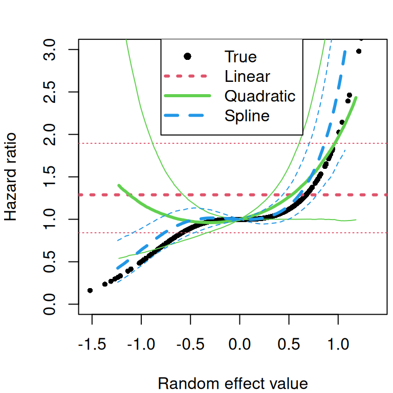
As expected, only the model with a spline effect is able to capture this complex non-linear effect. Of note, here both the Quadratic and Spline are not defined on the tails of the distribution (for rare/extreme values of the shared component) as they are defined based on the fitted values and despite having true values of the random effect as low as -1.5, fitted values are only reaching ~-1.2. One can extend the curves based on the random walk by assuming linearity from the last two points but it is not recommended to study areas of the distribution where we did not learn from the data, especially with random walks that are built on the data information directly.
Here for example, an individual with a high random effect compared to population average will be shifted to the right on the plot’s x-axis (where the population average location is at zero), meaning he experience higher risk associated with higher biomarker values. This plot shows how a shared component can have both a beneficial (i.e., HR<1) and deleterious (i.e., HR>1) effect on the risk, depending on its value, where the standard joint model gives a hazard ratio for the biomarker’s effect that includes 1, since it can only capture a beneficial or deleterious effect, not both simultaneously.
We can see how the goodness of fit metrics favors the spline association:
GOF <- data.frame("Linear" = c(M_jmSRE2$dic$dic, M_jmSRE2$waic$waic),
                  "Quadratic" = c(M_jmLSRE2$dic$dic, M_jmLSRE2$waic$waic),
                  "Spline" = c(M_jmNLSRE2$dic$dic, M_jmNLSRE2$waic$waic))
rownames(GOF) <- c("DIC", "WAIC");GOF
Linear Quadratic Spline
DIC 3855.775 3857.197 3841.008
WAIC 3857.632 3858.323 3850.068It is important to note that although these new models are validated by simulations (not published at the time of writing this book), it is easy to get into unstable estimates. Indeed, the level of flexibility and the complexity of this modeling approach needs sufficient data to perform well and can possibly lead to identifiability issues, therefore the use of these models should be supervised by experienced statisticians until more literature is available to support this methodology.
Of note, this framework to define non-linear associations also allows to consider time-dependent effects (\(\gamma(t)\)), although it has not yet been developed at the time of writing this book.
4.4 Joint model for multiple longitudinal and one survival outcome
So far we have explored joint models that integrate a single longitudinal outcome with a survival outcome but in many situations, researchers are interested in studying the relationship between multiple longitudinal outcomes and survival outcomes. For instance, in clinical studies, patients may have multiple biomarkers or clinical measurements taken over time, each of which may inform about the risk of an event, such as disease progression or death.
Joint models for multiple longitudinal and a survival outcome extend the traditional joint modeling framework to accommodate multiple time-varying markers. These models allow for the simultaneous analysis of several longitudinal trajectories and their effect on the survival outcome.
Let’s consider the following model: \[\begin{equation*} \left\{ \begin{array}{rl} \textrm{E}[Y_{1i}(t)]&= \eta_{1i}(t)\\ &= \beta_{10} + b_{1i0} + \beta_{11}\cdot t + \beta_{12}\cdot trt_i + \beta_{13}\cdot trt_i\cdot t\\ \log(\textrm{E}[Y_{2i}(t)])&= \eta_{2i}(t)\\ &= \beta_{20} + b_{2i0} + \beta_{21}\cdot t + \beta_{22}\cdot trt_i + \beta_{23}\cdot trt_i\cdot t\\ \lambda_i(t)&=\lambda_0(t)\exp\left(\gamma_1 \cdot \eta_{1i}(t)+ \gamma_2 \cdot \eta_{2i}(t)\right) \end{array} \right. \end{equation*}\] Here we consider two longitudinal outcomes, where the first is continuous and the second is counts, both influencing the risk of event through their current value, scaled by \(\gamma\) parameters.
We can simulate data from this model structure:
CV_i1 <- b_0 + b12 + b_1*time2 + b_2*trt2 + b_3*trt2*time2
CV_i1L <- b_0 + b1 + b_1*time + b_2*trtY + b_3*trtY*time
CV_i2 <- b_0 + b22 + b_1*time2 + b_2*trt2 + b_3*trt2*time2
CV_i2L <- b_0 + b2 + b_1*time + b_2*trtY + b_3*trtY*time
DatTmp <- permalgorithm(n, n_i2, Xmat=matrix(c(CV_i1, CV_i2), ncol=2),
                        betas=c(s_1, s_2)) # association
DatTmp2 <- DatTmp[which(!duplicated(DatTmp$Id, fromLast = T)),
                  c("Id","Event","Stop")]
datJM7_S <- data.frame(id = 1:n, eventTimes = mestime2[DatTmp2$Stop+1],
                       eventIndic = DatTmp2$Event, trt = trt)
datJM_Lt$Y1 <- rnorm(n_i*n, CV_i1L, b_e) # first outcome Gaussian
datJM_Lt$Y2 <- rpois(n_i*n, exp(CV_i2L)) # second outcome Poisson
datJM7_L <- datJM_Lt[-unlist(sapply(1:n, function(x)
  which(datJM_Lt$time>=datJM7_S$eventTimes[datJM7_S$id==x] &
        datJM_Lt$id==x))),]
As introduced in Section 3.4, we can include multiple longitudinal outcomes by setting the formula for longitudinal submodels formLong as a list of formulas, then the family argument is a vector. Since we have two markers, the association parameter assoc is now a vector and can accommodate different associations for each outcome (where an empty string means no association):
M_jmCV2 <- joint(formSurv = inla.surv(eventTimes, eventIndic) ~ -1,
                 formLong = list(Y1 ~ time * trt + (1 | id),
                                 Y2 ~ time * trt + (1 | id)),
                 dataSurv = datJM7_S, dataLong=datJM7_L,
                 family=c("gaussian", "poisson"), id="id",
                 timeVar="time", assoc=c("CV", "CV"))
summary(M_jmCV2)
Longitudinal outcome (L1, gaussian)
mean sd 0.025quant 0.5quant 0.975quant
Intercept_L1 1.0075 0.0686 0.8729 1.0075 1.1422
time_L1 -0.9967 0.0201 -1.0362 -0.9967 -0.9573
trt_L1 1.0912 0.1004 0.8943 1.0912 1.2881
time:trt_L1 0.4431 0.0390 0.3667 0.4431 0.5195
Res. err. (variance) 0.2356 0.0136 0.2101 0.2352 0.2634
Random effects variance-covariance (L1)
mean sd 0.025quant 0.5quant 0.975quant
Intercept_L1 1.0572 0.0762 0.9159 1.0543 1.2154
Longitudinal outcome (L2, poisson)
mean sd 0.025quant 0.5quant 0.975quant
Intercept_L2 1.0141 0.0574 0.9005 1.0145 1.1255
time_L2 -1.0537 0.0506 -1.1531 -1.0536 -0.9546
trt_L2 1.0045 0.0763 0.8554 1.0043 1.1550
time:trt_L2 0.5502 0.0605 0.4317 0.5502 0.6691
Random effects variance-covariance (L2)
mean sd 0.025quant 0.5quant 0.975quant
Intercept_L2 0.5005 0.0448 0.4189 0.4982 0.5949
Survival outcome
mean sd 0.025quant 0.5quant 0.975quant
Baseline risk (variance)_S1 0.5917 0.2169 0.2778 0.5545 1.1229
Association longitudinal - survival
mean sd 0.025quant 0.5quant 0.975quant
CV_L1_S1 0.5646 0.0862 0.3964 0.5641 0.7356
CV_L2_S1 0.2603 0.0975 0.0672 0.2606 0.4512
log marginal-likelihood (integration) log marginal-likelihood (Gaussian)
-26805.92 -26801.87
Deviance Information Criterion: 7941.063
Widely applicable Bayesian information criterion: 7928.919
Computation time: 10.24 secondsWe can see the summary of the fitted model includes the two longitudinal outcomes first followed by the survival outcome and the association parameters, where we have now two parameters corresponding to the two longitudinal outcomes. We can plot the posterior marginals of this model and compare with true values:
Plots_jm <- plot(M_jmCV2)
Plots_jm$Outcomes$L1$data <- rbind(Plots_jm$Outcomes$L1$data,
                                   Plots_jm$Outcomes$L2$data)
Plots_jm$Covariances$L1$data <- rbind(Plots_jm$Covariances$L1$data,
                                      Plots_jm$Covariances$L2$data)
ggarrange(eval(parse(text=P1)),
          ggarrange(eval(parse(text=P2)),
                    eval(parse(text=P3)), ncol=2), nrow=2,
          heights = c(1, 0.5))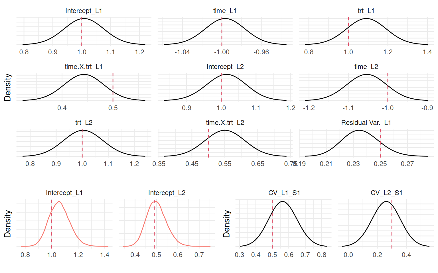
Here we assumed the two longitudinal markers are independent (i.e., we did not consider correlation between their random effects). We could include the correlation between random effects of the two longitudinal (here only random intercepts) by setting corLong=TRUE:
# since we simulated with covariance, we can verify
M_jmCV3 <- joint(formSurv = inla.surv(eventTimes, eventIndic) ~ -1,
                 formLong = list(Y1 ~ time * trt + (1 | id),
                                 Y2 ~ time * trt + (1 | id)),
                 dataSurv = datJM7_S, dataLong=datJM7_L, corLong=T,
                 family=c("gaussian", "poisson"), id="id",
                 timeVar="time", assoc=c("CV", "CV"))
Plots_jm <- plot(M_jmCV3)
eval(parse(text=P2))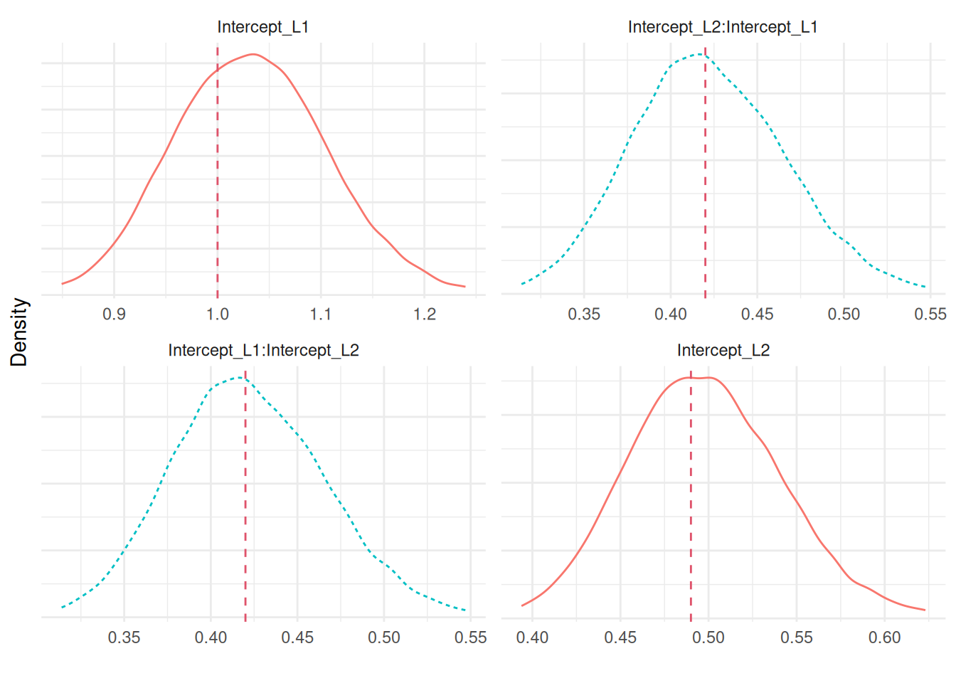
4.5 Joint model for multiple longitudinal and multiple survival outcomes
We now consider joint models that incorporate multiple longitudinal and multiple survival outcomes. For example in clinical research, patients may experience several types of events, such as disease recurrence, hospitalization, and death, each of which may be influenced by multiple longitudinal biomarkers or clinical measurements.
Let’s consider the following model, where the first event risk depends on the current value of a continuous and a count longitudinal marker while a second, different event risk depends on the random intercept from the continuous longitudinal marker: \[\begin{equation*} \left\{ \begin{array}{rl} \textrm{E}[Y_{1i}(t)]&= \eta_{1i}(t)\\ &= \beta_{10} + b_{1i0} + \beta_{11}\cdot t + \beta_{12}\cdot trt_i + \beta_{13}\cdot trt_i\cdot t \\ \log(\textrm{E}[Y_{2i}(t)])&= \eta_{2i}(t)\\ &= \beta_{20} + b_{2i0} + \beta_{21}\cdot t + \beta_{22}\cdot trt_i + \beta_{23}\cdot trt_i\cdot t\\ \lambda_{1i}(t)&=\lambda_{10}(t)\exp\left(\gamma_{11}\cdot \eta_{1i}(t)+ \gamma_{12}\cdot \eta_{2i}(t)\right)\\ \lambda_{2i}(t)&=\lambda_{20}(t)\exp\left(\gamma_{21}\cdot b_{1i0}\right) \end{array} \right. \end{equation*}\]
We can simulate data from this model (here we assume experiencing one event does not prevent from experiencing the other event, although we could also consider competing risks or multi-state models for multivariate survival outcomes):
DatTmp <- permalgorithm(n, n_i2, Xmat=matrix(b12, ncol=1), betas=c(s_1))
DatTmp2$Event2 <- DatTmp[which(!duplicated(DatTmp$Id, fromLast = T)),
                         "Event"]
DatTmp2$Stop2 <- DatTmp[which(!duplicated(DatTmp$Id, fromLast = T)),
                         "Stop"]
datJM8_S <- data.frame(id = 1:n, eventTimes = mestime2[DatTmp2$Stop+1],
                       eventTimes2 = mestime2[DatTmp2$Stop2+1],
                       eventIndic = DatTmp2$Event,
                       eventIndic2 = DatTmp2$Event2, trt = trt)
datJM8_L <- datJM_Lt[-unlist(sapply(1:n, function(x)
  which((datJM_Lt$time>=datJM8_S$eventTimes[datJM8_S$id==x] |
         datJM_Lt$time>=datJM8_S$eventTimes2[datJM8_S$id==x]) &
        datJM_Lt$id==x))),]
In order to fit the model, we need to supply a list of formulas for both the survival part (formSurv) and the longitudinal part (formLong). Moreover, the association is now set as a list of size 2 for the two longitudinal outcomes. Each element of the list is a vector of size 2 corresponding to the two survival outcomes. We set “CV” for current value association and “SRE_ind” to share only the random effect (as described in Section 4.3.2, “SRE” is used to share the time-dependent linear combination of random effects, while here we just share a time-fixed random intercept, which can be done with “SRE_ind” as shown in Section 4.3.1, although “SRE” would return similar results it is built differently to handle time dependence which is not necessary in this case).
M_jmCV4 <- joint(formSurv = list(inla.surv(eventTimes, eventIndic) ~ -1,
                                inla.surv(eventTimes2, eventIndic2) ~ -1),
                 formLong = list(Y1 ~ time * trt + (1 | id),
                                 Y2 ~ time * trt + (1 | id)),
                 dataSurv = datJM8_S, dataLong=datJM8_L, corLong=T,
                 family=c("gaussian", "poisson"), id="id",
                 timeVar="time", assoc=list(c("CV", "SRE_ind"),
                                            c("CV", "")))
summary(M_jmCV4, sdcor=T)
Longitudinal outcome (L1, gaussian)
mean sd 0.025quant 0.5quant 0.975quant
Intercept_L1 1.0318 0.0673 0.8999 1.0318 1.1639
time_L1 -0.9844 0.0311 -1.0454 -0.9844 -0.9234
trt_L1 1.0483 0.0954 0.8612 1.0483 1.2355
time:trt_L1 0.4316 0.0558 0.3223 0.4316 0.5410
Res. err. (sd) 0.4670 0.0184 0.4323 0.4665 0.5046
Longitudinal outcome (L2, poisson)
mean sd 0.025quant 0.5quant 0.975quant
Intercept_L2 1.0206 0.0575 0.9068 1.0210 1.1323
time_L2 -1.0065 0.0683 -1.1408 -1.0063 -0.8729
trt_L2 0.9822 0.0757 0.8341 0.9820 1.1313
time:trt_L2 0.4754 0.0824 0.3144 0.4752 0.6374
Random effects standard deviation / correlation
mean sd 0.025quant 0.5quant 0.975quant
Intercept_L1 1.0295 0.0367 0.9584 1.0290 1.1028
Intercept_L2 0.7128 0.0324 0.6515 0.7126 0.7776
Intercept_L1:Intercept_L2 0.5840 0.0403 0.4994 0.5863 0.6587
Survival outcome (S1)
mean sd 0.025quant 0.5quant 0.975quant
Baseline risk (variance)_S1 0.7384 0.1327 0.5128 0.7265 1.0336
Survival outcome (S2)
mean sd 0.025quant 0.5quant 0.975quant
Baseline risk (variance)_S2 0.3689 0.0938 0.2176 0.3579 0.5848
Association longitudinal - survival
mean sd 0.025quant 0.5quant 0.975quant
CV_L1_S1 0.5633 0.1019 0.3642 0.5629 0.7653
SRE_Intercept_L1_S2 0.5279 0.0729 0.3844 0.5279 0.6714
CV_L2_S1 0.2523 0.1195 0.0158 0.2527 0.4862
log marginal-likelihood (integration) log marginal-likelihood (Gaussian)
-27198.84 -27192.07
Deviance Information Criterion: 8853.459
Widely applicable Bayesian information criterion: 8823.71
Computation time: 19.1 secondsWe can have a look at the marginal posteriors and compare to true values (with the dashed red line indicating the true value):
Plots_jm <- plot(M_jmCV4)
Plots_jm$Outcomes$L1$data <- rbind(Plots_jm$Outcomes$L1$data,
                                   Plots_jm$Outcomes$L2$data)
ggarrange(eval(parse(text=P1)),
          ggarrange(eval(parse(text=P2)),
                    eval(parse(text=P3)), ncol=2), nrow=2,
          heights = c(1, 0.5))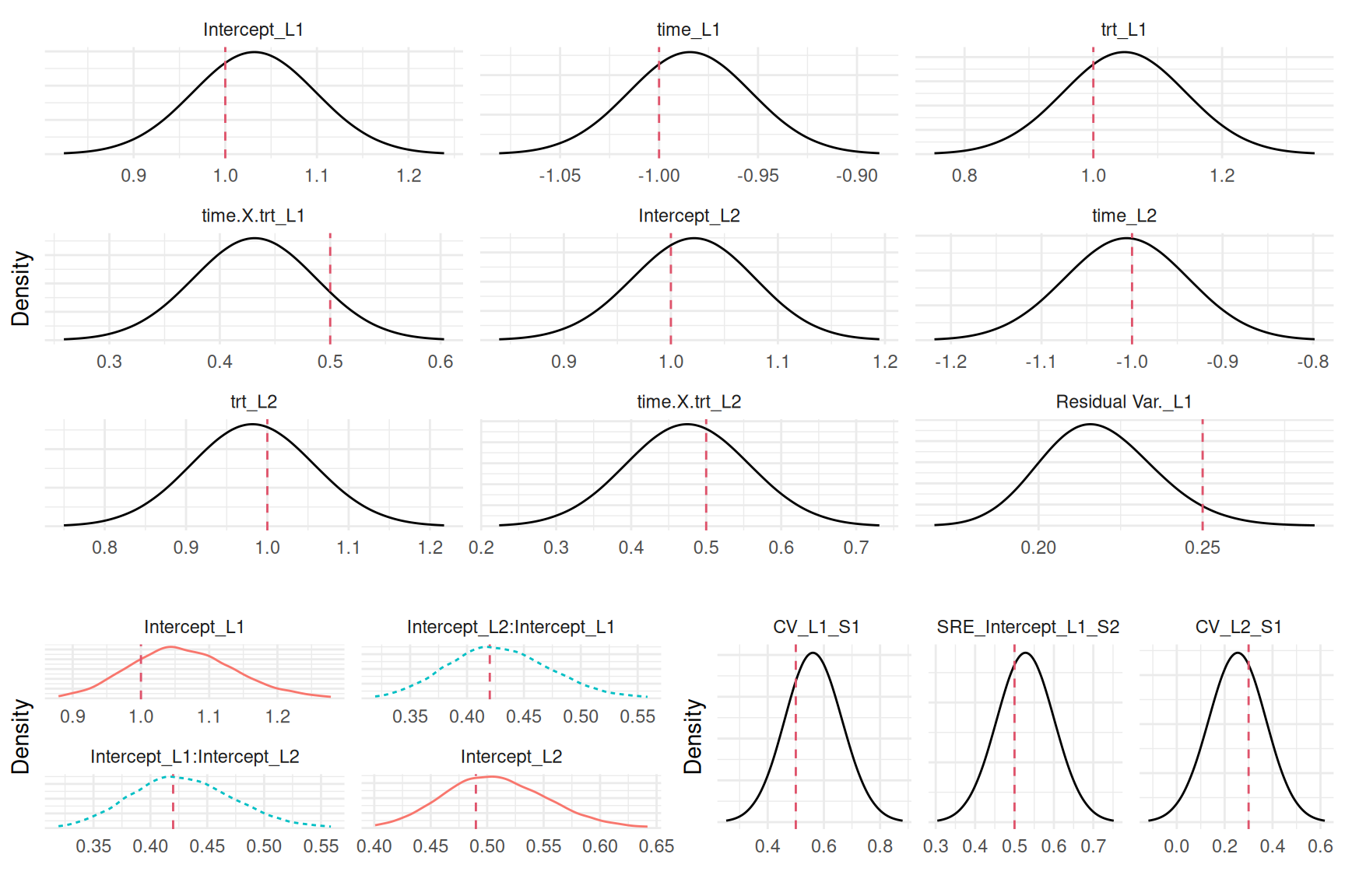
4.5.1 Real-data application: multivariate outcomes in the PBC clinical trial
Throughout this book, the theoretical and practical aspects of survival, longitudinal, and joint models have been developed using a range of illustrative examples. To conclude this chapter, we demonstrate the full capabilities of the INLAjoint package on a problem that reflects the true complexity of a clinical trial. The Primary Biliary Cholangitis (PBC) dataset has been used to illustrate some concepts in the book so far. In Chapter 1, we compared the performance of INLA with MCMC for a basic joint model. In Chapter 2, it helped illustrating the assumptions of baseline hazard approximation in survival analysis. While these examples were instructive, they only scratched the surface of the clinical and statistical richness this dataset offers. The true complexity of a clinical trial like the PBC study lies in its multivariate structure, which we will now explore to showcase the joint modeling framework implemented in INLAjoint.
The PBC dataset contains longitudinal information from 312 randomized patients followed at the Mayo Clinic between 1974 and 1988 (Murtaugh et al. (1994)). A comprehensive analysis of this disease requires monitoring a panel of biomarkers that capture different aspects of the disease process. The dataset includes repeated measurements for more than seven longitudinal markers, including: serum bilirubin (lognormal), platelets (Poisson), SGOT (aspartate aminotransferase, lognormal), albumin (Gaussian), ascites (binomial), spiders (binomial), and prothrombin time (Gaussian). Furthermore, patients in the trial are assumed at risk of two competing events: death and liver transplantation. Of note, this application is only for illustrative purpose and does not meet clinical standards for modeling. A formal clinical study would require a more rigorous process of variable selection, in-depth validation, and direct collaboration with medical experts to ensure all assumptions and interpretations align with current medical knowledge and practice.
Analyzing these multiple outcomes separately would be statistically inefficient and clinically misleading. The biomarkers are interconnected indicators of a single, complex process. For instance, an increase in serum bilirubin levels and a decrease in albumin levels are both markers of deteriorating liver function. Similarly, death and transplantation are not independent events. A separate analysis would fail to capture the correlation between biomarker trajectories and would be unable to properly account for the informative censoring that occurs when a patient’s longitudinal follow-up is terminated by a survival event.
The objective is to construct a comprehensive joint model that includes nine outcomes, based on the developments described in this book, including: a competing-risk survival model (Section 2.8), generalized linear mixed models for various outcome types (Section 3.3), and a sophisticated set of association structures (Section 4.3). By doing so, this section will showcase the practical feasibility of using INLA and the INLAjoint package to address complex, real-world research questions that lie beyond the scope of traditional statistical software. A multivariate joint model allows to understand the disease by modeling interdependencies between outcomes explicitly. This approach provides a powerful framework to assess how multiple, simultaneous biomarker trajectories collectively influence the risk of competing clinical outcomes.
We specify a joint model that includes seven longitudinal submodels and two risk-specific survival submodels. The structure of this nine-outcome model aims to represent the clinical hypotheses about primary biliary cholangitis, where various aspects of liver function and general health are believed to influence patient prognosis.
This serves as an illustration of a complex model where we can have multiple longitudinal outcomes that include non-linear functions of time and multiple random effects. For this illustrative example, the longitudinal models for most outcomes are kept simple (e.g., a single random intercept) to reduce computational burden. However, nothing prevents the inclusion of multiple groups of multiple random effects assuming independent longitudinal markers, or a large variance-covariance for all the random effects in the model when assuming longitudinal markers are correlated. As of now, INLAjoint can handle up to 24 correlated random effects, and even more could be handled, though a very large number of parameters would be difficult to interpret and would require a substantial amount of data for proper estimation (however, multiple groups of up to 24 correlated random effects could be considered in a joint model and the extension to more than 24 correlated random effects is straightforward and could be implemented upon request). Thus, the model showcases the high level of complexity that we can deal with, even while limiting the number of random effects for this specific application. The full model is presented below:
Serum bilirubin - lognormal \[\begin{align*} \textrm{E}[Y_{i1}(t)] &= \eta_{i1}(t)\\ &= (\beta_{10} + b_{i10}) + \beta_{11} \cdot f_1(t) + \beta_{12} \cdot f_2(t) + (\beta_{13} + b_{i13}) \cdot f_1(t) + (\beta_{14} + b_{i14}) \cdot f_2(t) \end{align*}\] where \(f1(t)\) and \(f2(t)\) represent the basis functions of natural cubic splines.
Platelet - Poisson \[\begin{align*} \log(\textrm{E}[Y_{i2}(t)]) &= \eta_{i2}(t)\\ &= (\beta_{20} + b_{i20})+(\beta_{21}+b_{i21}) \cdot t+\beta_{22} \cdot drug_i + \beta_{23} \cdot sex_i + \beta_{24} \cdot drug_i\cdot t + \\ & \quad \quad \beta_{25} \cdot sex_i\cdot t + \beta_{26} \cdot drug_i\cdot sex_i + \beta_{27} \cdot drug_i\cdot sex_i\cdot t \end{align*}\]
Aspartate aminotransferase SGOT - lognormal \[\begin{align*} \textrm{E}[Y_{i3}(t)]&= \eta_{i3}(t) \\ &= (\beta_{30} + b_{i30})+\beta_{31} \cdot t \end{align*}\]
Albumin - Gaussian \[\begin{align*} \textrm{E}[Y_{i4}(t)] &= \eta_{i4}(t) \\ &= (\beta_{40} + b_{i40})+\beta_{41} \cdot t \end{align*}\]
Ascites - Binomial \[\begin{align*} \textrm{logit}(\textrm{E}[Y_{i5}(t)]) &= \eta_{i5}(t)\\ &= (\beta_{50} +b_{i50})+\beta_{51} \cdot t \end{align*}\]
Spiders - Binomial \[\begin{align*} \textrm{logit}(\textrm{E}[Y_{i6}(t)]) &= \eta_{i6}(t)\\ &= (\beta_{60} +b_{i60})+\beta_{61} \cdot t \end{align*}\]
Prothrombin - Gaussian \[\begin{align*} \textrm{E}[Y_{i7}(t)] &= \eta_{i7}(t) \\ &= (\beta_{70} +b_{i70})+\beta_{71} \cdot t \end{align*}\]
Death risk \[\begin{align*} \lambda_{i1}(t) &= \lambda_{01}(t)\ \textrm{exp}\left(\gamma_{11} \cdot \eta_{i1}(t) + \gamma_{12} \cdot \eta_{i2}(t)+ \gamma_{13} \cdot b_{i50} + \gamma_{14} \cdot \frac{\partial \eta_{i2}(t)}{\partial t}\right) \end{align*}\]
Transplantation risk \[\begin{align*} \lambda_{i2}(t) &= \lambda_{02}(t)\ \textrm{exp}\left(\gamma_{21} \cdot \eta_{i2}(t) + \gamma_{22} \cdot \eta_{i3}(t) + \gamma_{23} \cdot b_{i40} + \gamma_{24} \cdot \eta_{i6}(t) + \gamma_{25} \cdot \frac{\partial \eta_{i6}(t)}{\partial t}\right) \end{align*}\]
This complex joint model is structured to showcase the flexibility of the INLAjoint framework. The first mixed-effects model, for serum bilirubin, shows the ability to handle natural cubic splines associated with both fixed and random effects, allowing to capture flexible, non-linear individual trajectories over time. In contrast, the second mixed-effects model for platelet illustrates the capacity to manage complex covariate structures by including a triple interaction term. The remaining longitudinal models are intentionally kept simple, incorporating only a random intercept and a fixed linear slope to balance complexity with computational efficiency. Finally, the association between the longitudinal and survival components relies on diverse parametrizations, including the current value (CV), current slope (CS), and shared random effects (SRE) to highlight the versatility of INLAjoint in specifying nuanced, clinically-driven hypotheses. The complete structure of this nine-outcome model is summarized in the table below for clarity:
| Outcome | Model | Association with death risk | Association with transplantation risk |
|---|---|---|---|
| Serum bilirubin | Lognormal mixed model | Current value (CV) | None |
| Platelets | Poisson mixed model | Current value and slope (CV_CS) | Current value |
| SGOT | Lognormal mixed model | None | Current value |
| Albumin | Gaussian mixed model | None | Shared random effect (SRE) |
| Ascites | Binomial mixed model | Shared random effect | None |
| Spiders | Binomial mixed model | None | Current value and slope |
| Prothrombin time | Gaussian mixed model | Current slope (CS) | None |
| Death | Proportional hazards (RW2) | – | – |
| Transplantation | Proportional hazards (RW2) | – | – |
INLAjoint provides a simplified syntax that handles the complexity of data structuring and model construction required for R-INLA, allowing the user to specify this entire nine-outcome model with a few lines of code.
First, the data is prepared by selecting the relevant variables and defining the natural spline basis functions of time.
library(JMbayes2)
pbc2_2 <- pbc2[, c("id", "drug", "sex", "year", "ascites", "spiders",
                   "serBilir", "albumin", "SGOT", "platelets",
                   "prothrombin")]
pbc2.id$death <- ifelse(pbc2.id$status=="dead", 1, 0)
pbc2.id$tsp <- ifelse(pbc2.id$status=="transplanted", 1, 0)
BSP <- ns(pbc2_2$year, knots=1)
f1 <- function(x) predict(BSP, x)[,1]
f2 <- function(x) predict(BSP, x)[,2]
The entire joint model is then fitted with a single call to the joint() function:
IJ2 <- joint(formSurv = list(inla.surv(years, death) ~ 1,
                             inla.surv(years, tsp) ~ 1),
             formLong = list(serBilir ~  f1(year) + f2(year) +
                                         (1 + f1(year) + f2(year) |id),
                            platelets ~ year * drug * sex + (1 + year|id),
                            SGOT ~ year + (1|id),
                            albumin ~ year + (1|id),
                            ascites ~ year + (1|id),
                            spiders ~ year + (1|id),
                            prothrombin ~ year + (1|id)),
             dataLong = pbc2_2, dataSurv = pbc2.id, id = "id",
             timeVar = "year", basRisk="rw2", corLong=TRUE,
             family = c("lognormal", "poisson", "lognormal", "gaussian",
                        "binomial", "binomial", "lognormal"),
             assoc = list(c("CV", ""), c("CV", "CV"), c("", "CV"),
                          c("", "SRE_ind"), c("SRE_ind", ""),
                          c("", "CV_CS"), c("CS", "")),
             control=list(int.strategy="eb"))
print(summary(IJ2))
Longitudinal outcome (L1, lognormal)
mean sd 0.025quant 0.5quant 0.975quant
Intercept_L1 0.5181 0.0577 0.4051 0.5181 0.6312
f1year_L1 2.2896 0.1399 2.0153 2.2896 2.5638
f2year_L1 2.3901 0.1881 2.0214 2.3901 2.7588
Res. err. (variance) 0.0926 0.0038 0.0854 0.0925 0.1003
Longitudinal outcome (L2, poisson)
mean sd 0.025quant 0.5quant 0.975quant
Intercept_L2 5.4626 0.0927 5.2809 5.4626 5.6443
year_L2 -0.1207 0.0486 -0.2160 -0.1207 -0.0255
drugDpenicil_L2 -0.0511 0.1210 -0.2881 -0.0511 0.1860
sexfemale_L2 0.0661 0.0972 -0.1243 0.0661 0.2566
year:drugDpenicil_L2 -0.0271 0.0637 -0.1520 -0.0271 0.0978
year:sexfemale_L2 0.0657 0.0510 -0.0343 0.0657 0.1656
drugDpenicil:sexfemale_L2 -0.0154 0.1284 -0.2671 -0.0154 0.2363
year:drugDpenicil:sexfemale_L2 -0.0215 0.0676 -0.1540 -0.0215 0.1110
Longitudinal outcome (L3, lognormal)
mean sd 0.025quant 0.5quant 0.975quant
Intercept_L3 4.7237 0.0280 4.6688 4.7237 4.7786
year_L3 -0.0045 0.0027 -0.0097 -0.0045 0.0007
Res. err. (variance) 0.0943 0.0033 0.0881 0.0943 0.1009
Longitudinal outcome (L4, gaussian)
mean sd 0.025quant 0.5quant 0.975quant
Intercept_L4 3.5153 0.0246 3.4672 3.5153 3.5635
year_L4 -0.0763 0.0030 -0.0821 -0.0763 -0.0705
Res. err. (variance) 0.1218 0.0042 0.1139 0.1217 0.1303
Longitudinal outcome (L5, binomial)
mean sd 0.025quant 0.5quant 0.975quant
Intercept_L5 -4.6129 0.2292 -5.0622 -4.6129 -4.1636
year_L5 0.4451 0.0346 0.3774 0.4451 0.5129
Longitudinal outcome (L6, binomial)
mean sd 0.025quant 0.5quant 0.975quant
Intercept_L6 -1.4075 0.1728 -1.7462 -1.4075 -1.0688
year_L6 0.1695 0.0254 0.1197 0.1695 0.2193
Longitudinal outcome (L7, lognormal)
mean sd 0.025quant 0.5quant 0.975quant
Intercept_L7 2.3681 0.0065 2.3554 2.3681 2.3809
year_L7 0.0132 0.0007 0.0118 0.0132 0.0146
Res. err. (variance) 0.0069 0.0002 0.0065 0.0069 0.0074
Random effects variance-covariance
mean sd 0.025quant 0.5quant 0.975quant
Intercept_L1 1.0352 0.1117 0.8526 1.0250 1.2897
f1year_L1 4.3268 0.6358 3.2099 4.2780 5.7458
f2year_L1 4.1200 0.9049 2.6495 4.0258 6.1997
Intercept_L2 0.1527 0.0125 0.1306 0.1523 0.1791
year_L2 0.0319 0.0042 0.0244 0.0316 0.0410
Intercept_L3 0.2157 0.0198 0.1812 0.2139 0.2582
Intercept_L4 0.1453 0.0140 0.1210 0.1444 0.1754
Intercept_L5 7.5851 1.4691 5.0489 7.4929 10.7468
Intercept_L6 6.0018 0.9099 4.4734 5.9055 7.9241
Intercept_L7 0.0108 0.0010 0.0091 0.0108 0.0129
Intercept_L1:f1year_L1 0.7088 0.2110 0.3246 0.6986 1.1610
Intercept_L1:f2year_L1 0.5771 0.3435 -0.0918 0.5719 1.2515
Intercept_L1:Intercept_L2 -0.0786 0.0255 -0.1314 -0.0777 -0.0330
Intercept_L1:year_L2 -0.0210 0.0134 -0.0490 -0.0206 0.0045
Intercept_L1:Intercept_L3 0.2963 0.0379 0.2279 0.2945 0.3767
Intercept_L1:Intercept_L4 -0.2245 0.0301 -0.2868 -0.2230 -0.1685
Intercept_L1:Intercept_L5 1.7924 0.2882 1.3064 1.7750 2.4219
Intercept_L1:Intercept_L6 1.2382 0.2125 0.8818 1.2238 1.7108
Intercept_L1:Intercept_L7 0.0495 0.0071 0.0369 0.0491 0.0653
f1year_L1:f2year_L1 1.7538 0.6425 0.5703 1.7017 3.1539
f1year_L1:Intercept_L2 -0.1199 0.0613 -0.2452 -0.1184 0.0023
f1year_L1:year_L2 -0.0420 0.0342 -0.1121 -0.0422 0.0250
f1year_L1:Intercept_L3 0.4384 0.0808 0.2933 0.4322 0.6141
f1year_L1:Intercept_L4 -0.4606 0.0767 -0.6218 -0.4575 -0.3192
f1year_L1:Intercept_L5 4.3957 0.7409 3.0465 4.3567 5.9524
f1year_L1:Intercept_L6 2.2738 0.5061 1.3103 2.2525 3.3457
f1year_L1:Intercept_L7 0.0903 0.0178 0.0580 0.0900 0.1255
f2year_L1:Intercept_L2 -0.0434 0.0840 -0.2154 -0.0450 0.1186
f2year_L1:year_L2 -0.0650 0.0401 -0.1485 -0.0638 0.0111
f2year_L1:Intercept_L3 0.2367 0.1078 0.0310 0.2344 0.4454
f2year_L1:Intercept_L4 -0.3587 0.1039 -0.5737 -0.3594 -0.1582
f2year_L1:Intercept_L5 2.8274 0.9543 1.0341 2.7901 4.7214
f2year_L1:Intercept_L6 1.2333 0.6779 -0.0908 1.2375 2.6137
f2year_L1:Intercept_L7 0.0432 0.0230 -0.0024 0.0433 0.0896
Intercept_L2:year_L2 -0.0043 0.0048 -0.0139 -0.0044 0.0050
Intercept_L2:Intercept_L3 -0.0068 0.0110 -0.0293 -0.0063 0.0143
Intercept_L2:Intercept_L4 0.0419 0.0097 0.0231 0.0418 0.0611
Intercept_L2:Intercept_L5 -0.3797 0.0831 -0.5534 -0.3734 -0.2342
Intercept_L2:Intercept_L6 -0.2204 0.0682 -0.3621 -0.2164 -0.0936
Intercept_L2:Intercept_L7 -0.0134 0.0024 -0.0184 -0.0132 -0.0089
year_L2:Intercept_L3 -0.0145 0.0056 -0.0257 -0.0142 -0.0039
year_L2:Intercept_L4 0.0071 0.0052 -0.0032 0.0071 0.0178
year_L2:Intercept_L5 -0.0693 0.0453 -0.1656 -0.0669 0.0157
year_L2:Intercept_L6 -0.0213 0.0350 -0.0885 -0.0217 0.0521
year_L2:Intercept_L7 -0.0010 0.0013 -0.0034 -0.0009 0.0014
Intercept_L3:Intercept_L4 -0.0714 0.0125 -0.0979 -0.0708 -0.0485
Intercept_L3:Intercept_L5 0.6401 0.1184 0.4445 0.6302 0.8964
Intercept_L3:Intercept_L6 0.4803 0.0905 0.3205 0.4711 0.6756
Intercept_L3:Intercept_L7 0.0138 0.0030 0.0084 0.0136 0.0201
Intercept_L4:Intercept_L5 -0.8013 0.1103 -1.0336 -0.7962 -0.6122
Intercept_L4:Intercept_L6 -0.4772 0.0784 -0.6500 -0.4720 -0.3369
Intercept_L4:Intercept_L7 -0.0197 0.0026 -0.0252 -0.0196 -0.0149
Intercept_L5:Intercept_L6 4.5313 0.7441 3.2431 4.4920 6.1519
Intercept_L5:Intercept_L7 0.1574 0.0237 0.1160 0.1563 0.2089
Intercept_L6:Intercept_L7 0.1077 0.0177 0.0756 0.1067 0.1440
Survival outcome (S1)
mean sd 0.025quant 0.5quant 0.975quant
Baseline risk (variance)_S1 0.0201 0.0191 0.0012 0.0144 0.0714
Survival outcome (S2)
mean sd 0.025quant 0.5quant 0.975quant
Baseline risk (variance)_S2 0.2584 0.1963 0.0588 0.2023 0.7969
Association longitudinal - survival
mean sd 0.025quant 0.5quant 0.975quant
CV_L1_S1 1.4731 0.1475 1.1865 1.4717 1.7673
CV_L2_S1 -0.7161 0.1584 -1.0311 -0.7150 -0.4075
CV_L2_S2 -0.4598 0.2616 -0.9707 -0.4612 0.0591
CV_L3_S2 -0.0346 0.4170 -0.8581 -0.0337 0.7836
SRE_Intercept_L4_S2 0.9846 0.2689 0.4540 0.9850 1.5126
SRE_Intercept_L5_S1 -0.1336 0.1640 -0.4597 -0.1324 0.1859
CV_L6_S2 0.1020 0.1082 -0.1082 0.1010 0.3177
CS_L6_S2 -0.5658 1.5039 -3.7943 -0.4757 2.0855
CS_L7_S1 0.1353 1.4423 -2.6828 0.1280 2.9960
log marginal-likelihood (integration) log marginal-likelihood (Gaussian)
-85336.08 -85271.46
Deviance Information Criterion: 54487.67
Widely applicable Bayesian information criterion: 79989.37
Computation time: 914.56 secondsThe arguments formSurv and formLong are lists defining the formulas for each outcome, the family vector gives the family for each longitudinal model and the assoc list defines the association between the longitudinal and survival components. The choice of control = list(int.strategy = "eb") switches from default hyperparameter integration to the empirical Bayes strategy (see Section 1.5.1) to accelerate computations while maintaining good frequentist properties, as supported by simulation studies (Rustand, Van Niekerk, et al. (2024)).
A model of this dimension pushes the boundaries of what is feasible with traditional methods. Sampling-based approaches like MCMC would require hours to achieve convergence, if they converge at all. The INLA methodology provides a stable, accurate, and fast alternative
By examining the association parameters that quantify the strength of the relationship between each biomarker and the risk of events, we can translate these statistical results into clinically meaningful insights. For example, the current value of serum bilirubin (CV_L1_S1) is a strong and significant predictor of death. The positive coefficient indicates that higher current levels of bilirubin are associated with an increased hazard of death. Similarly, the current value of platelet counts (CV_L2_S1) shows a negative association with the death hazard through the shared random effect, suggesting that patients with a higher platelet counts are at lower risk of death.
Among the association parameters for the risk of transplantation, SRE_Intercept_L4_S2 shows a statistically significant positive association with the random intercept of albumin. The remaining parameters are not statistically significant, as their 95% credible intervals all contain zero. This is likely the result of the small sample size (e.g., only 29 events recorded for transplantation), and a larger sample could reveal more significant associations between the longitudinal markers and the risk of transplantation.
This detailed analysis showcases how a multivariate joint model can successfully fit the complex effects of multiple biomarkers on competing clinical endpoints.
Let’s now consider some dynamic predictions based on this model. We assume a new individual has longitudinal measurements of all biomarkers up to two different landmark times. We also consider another individual to illustrate individual-specific predictions. For simplicity, these new individual’s data come from the training dataset but they are treated as new data. The data for predictions is then:
Ndata <- rbind(pbc2_2[pbc2_2$id == 32,],
               pbc2_2[pbc2_2$id == 32,],
               pbc2_2[pbc2_2$id == 19,]) # all the data
Ndata$id <- c(rep("Individual 1 (landmark 1)", 16),
              rep("Individual 1 (landmark 2)", 16),
              rep("Individual 2", 15))
NewData <- Ndata[-c(6:16, 27:32, 38:47),];NewData
id drug sex year ascites spiders serBilir
1 Individual 1 (landmark 1) placebo female 0.0000000 No No 1.8
2 Individual 1 (landmark 1) placebo female 0.4983025 No No 1.9
3 Individual 1 (landmark 1) placebo female 0.9966050 No No 1.6
4 Individual 1 (landmark 1) placebo female 1.9932099 No No 1.3
5 Individual 1 (landmark 1) placebo female 3.0089804 No No 1.4
17 Individual 1 (landmark 2) placebo female 0.0000000 No No 1.8
18 Individual 1 (landmark 2) placebo female 0.4983025 No No 1.9
19 Individual 1 (landmark 2) placebo female 0.9966050 No No 1.6
20 Individual 1 (landmark 2) placebo female 1.9932099 No No 1.3
21 Individual 1 (landmark 2) placebo female 3.0089804 No No 1.4
22 Individual 1 (landmark 2) placebo female 4.0055854 No No 1.2
23 Individual 1 (landmark 2) placebo female 4.9885007 No No 1.2
24 Individual 1 (landmark 2) placebo female 5.9987953 No No 1.0
25 Individual 1 (landmark 2) placebo female 6.9762348 No No 1.0
26 Individual 1 (landmark 2) placebo female 8.1069981 No No 0.7
33 Individual 2 D-penicil female 0.0000000 No No 0.7
34 Individual 2 D-penicil female 0.5311576 No Yes 0.5
35 Individual 2 D-penicil female 1.1061220 No No 0.5
36 Individual 2 D-penicil female 1.9630928 No No 0.5
37 Individual 2 D-penicil female 2.9596977 No Yes 0.3 albumin SGOT platelets prothrombin
1 3.34 82.6 286 10.6
2 4.05 116.3 223 10.5
3 4.03 96.1 241 11.5
4 3.50 89.9 225 10.1
5 4.08 107.0 250 10.6
17 3.34 82.6 286 10.6
18 4.05 116.3 223 10.5
19 4.03 96.1 241 11.5
20 3.50 89.9 225 10.1
21 4.08 107.0 250 10.6
22 3.82 91.5 238 9.9
23 3.70 99.2 176 9.6
24 3.49 89.9 176 9.9
25 3.49 91.5 192 10.7
26 3.32 83.0 178 9.7
33 3.56 93.0 209 11.0
34 4.00 46.5 215 11.2
35 4.11 58.9 205 10.4
36 4.46 49.6 191 10.4
37 4.30 60.5 218 10.2 We can now compute predictions based on this new data and plot the results. We limit the plots to serum bilirubin and platelet counts but all the markers included in the model have predictions in P$predL. We only focus on these for simplicity and because other models are kept simple with only linear trends.
P <- predict(IJ2, NewData, horizon = 14, CIF=TRUE,
             inv.link=TRUE, resErrLong = TRUE)
P$PredLSB <- P$PredL[P$PredL$Outcome=="serBilir",]
P$PredLP <- P$PredL[P$PredL$Outcome=="platelets",]
library(ggpubr)
ggarrange(ggplot(P$PredLSB, aes(x = year, y = quant0.5)) +
            geom_point(data=Ndata, aes(x=year, y=serBilir), col=80) +
            geom_line() + scale_y_log10() +
            geom_ribbon(aes(ymin=quant0.025, ymax=quant0.975), alpha=0.1)+
            geom_point(data=NewData, aes(x=year, y=serBilir)) +
            ylab("Serum bilirubin") + facet_wrap(~id),
          ggplot(P$PredLP, aes(x = year, y = quant0.5)) +
            geom_point(data=Ndata, aes(x=year, y=platelets), col=80) +
            geom_line() + scale_y_log10() +
            geom_ribbon(aes(ymin=quant0.025, ymax=quant0.975), alpha=0.1)+
            geom_point(data=NewData, aes(x=year, y=platelets)) +
            ylab("Platelets count") + facet_wrap(~id),
          ggplot(P$PredS, aes(x = year, y = CIF_quant0.5, colour=Outcome,
                              linetype=Outcome)) + geom_line() +
            geom_ribbon(aes(ymin=CIF_quant0.025, ymax=CIF_quant0.975),
                        alpha=0.1) + coord_cartesian(ylim = c(0, 0.5)) +
            theme(legend.position="none") + ylab("Event probability") +
            facet_wrap(~id), ncol=1)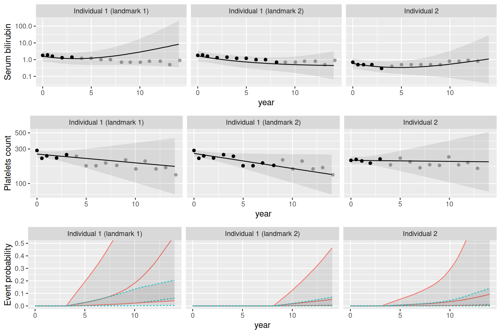
predict function to compute conditional predictions. Gray points are future observations not taken into account in the computations of the predictions. Top is serum bilirum levels on the log scale, middle is platelets counts and bottom are event probability based on cumulative incidence functions for competing risks of death (straight line) and transplantation (dashed line).
We can see how the individual 1 prediction at first landmark is aligned with the observations supplied and slightly misses the future (unknown) trend given by future observations of serum bilirubin, although the 95% interval includes these points, meaning they are plausible according to our predictions. Updating the predictions for this individual once more measurements are recorded is straightforward as illustrated in the second column of plots in Figure 4.18. The event probabilities (death and transplantation) are computed, assuming the individual was event free at the last longitudinal measurement provided to the survival function. Keep in mind there are 5 other longitudinal markers in the model, not shown here because we kept them very simple (only random intercept and linear trend over time), making them less interesting to represent in this specific context. However, the predictions are computed based on the entire 9 outcome model and the predicted trajectory of each outcome is available in the output of predict().
4.6 Priors for association parameters
The priors for the association parameters are quite straightforward, since they usually are considered as fixed effects, they are assigned a zero-centered Gaussian distribution. For the association SRE_ind, the argument priorSRE_ind can be set in control options of the joint() function. It is a list with mean and precision for the Gaussian prior distribution on the association of independent random effects. Default is list(mean=0, prec=1). The reason why this association parameter have its own prior is based on performances in simulations, these parameters are associated to constant variables while other association parameters described are associated to variables that can be time varying, so they are handled differently, internally.
The argument priorAssoc is used to set the prior distribution of association parameters for “SRE”, CV” and “CS” associations. It is a list with mean and precision for the Gaussian prior distribution of the association parameters. Default is list(mean=0, prec=0.01). Initial value for all the association parameters can be set with the argument assocInit (default value is 0.1), although initial values have negligible impact with INLA in most situations. The prior for the cumulative value association is directly set within the R-INLA framework, as shown in Section 4.3.6 where we used the same default values as for “CV”.
For non-linear associations, priors can be set for the mean, the slope and the splines. The argument NLpriorAssoc in control options includes 3 options: mean, slope and spline, each including 3 options: mean for the mean of the prior, prec for the precision of the prior and initial for the initial value.