In this chapter, we give a comprehensive introduction to some survival models that can be fitted with INLA, along with illustrative examples based on simulated data. Most survival models used in practice by clinicians, epidemiologists and biostatisticians can be fitted with this method and the user-friendly R package INLAjoint makes this accessible to a wide audience. The models presented include the Cox proportional hazards, accelerated failure time, stratified proportional hazards, mixture cure, competing risks, multi-state, frailty and shared frailty joint models. We show how censoring and truncation mechanisms can be handled (e.g., right censoring, interval censoring, left truncation), and various baseline hazard options (e.g., parametric with exponential, Weibull or Gompertz, as well as semi-parametric with random walks) are accommodated. Each model is described, illustrated with a fully reproducible example, interpreted, and some key quantities and figures are computed to show how to extract information efficiently.
Overview of survival models presented in this chapter.
Model
Assumption
Purpose
Section
Proportional Hazards
Exponential
Constant hazard over time
Simple baseline when risk is time-invariant
2.2.1
Weibull
Monotonically increasing/decreasing hazard
More flexibility compared to exponential but still strong assumption on the baseline hazard’s shape
2.2.2
Semi-parametric (random walks)
Smooth but flexible hazard shape
When baseline hazard shape is unknown
2.2.3
Specialized Models
Stratified PH
Proportional hazards within strata, different baselines between strata
Controlling for a categorical variable that violates PH
2.6
Mixture Cure
Population is a mix of “cured” and “at-risk” individuals
Analyzing data with a long-term survivor plateau
2.7
Competing Risks
Multiple event types censoring each other
Analyzing cause-specific event risks
2.8
Multi-state
Subjects transition through multiple transient/absorbing states
Modeling complex disease progression pathways
2.9
Frailty Model
Unobserved factors create heterogeneity in risk
Analyzing clustered data or recurrent events
2.10
Joint Frailty Model
Frailty is shared between two or more survival processes
Modeling the association between different event times
2.11
2.1 Introduction
In survival analysis, the outcome corresponds to the time elapsed until an event of interest occurs. Some patients will observe the event while other patients may not. When the follow-up of the study is over, remaining patients are censored. Some patients leave the study early (i.e., before the end of follow-up), they are lost to follow-up and considered censored at their last visit. The event is usually death, but other events of interest (e.g., progression of a disease) can be analyzed with survival models. The shape of the distribution of survival times justifies the requirement for specific models, because survival times are always positive, they often have skewed shapes of distribution and thus, statistical methods that rely on normality are not directly applicable and may produce invalid results with survival data. However, a suitable transformation of the event times, such as the logarithm or the square root can help with this issue. The main specificity in the analysis of survival times is censoring (i.e., the event is only observed for some patients).
Censoring can be categorized as follows:
Right censoring: The event time occurs after the last time point of observation.
Left censoring: The event time occurs before the first time point of observation.
Interval censoring: The event of interest is only known to occur between two time points.
Another way to classify censoring focuses on the relationship between the probability of a subject being censored and the risk of event:
Informative censoring: The risk of event for individuals in the study is different from the risk of event from censored individuals (it is similar to the “missing not at random” missing data mechanism introduced in Section 3.1).
Examples: Patient decides to stop taking the treatment because of side effects; Patient is too sick and clinicians decide to switch to another treatment (assuming independent censoring in this case would lead to underestimation of the hazard); Patient feels cured by an effective treatment and may no longer feel the need to follow-up (assuming independent censoring in this case would lead to overestimation of the hazard).
Non-informative (or random) censoring: The individual withdraws from the study for reasons not related to the study (It is similar to the “missing completely at random” missing data mechanism introduced in Section 3.1).
Examples: The event has not occurred at the end of the follow-up; Patient moves to another country and cannot continue its participation to the trial.
Censoring due to loss of follow-up should be non-informative to reduce the bias in the estimates of survival curves (i.e., the censoring time is statistically independent from the event time). For example in a clinical trial where we study disease progression as an event, drop-out can occur when the disease progression leads a patient to die or withdraw from the trial to seek other treatment options, the drop-out is then informative for the estimation of the disease progression. If the disease progression correlates with a biomarker that is being monitored, modeling the disease progression separately from the drop-out process may be inefficient and lead to biased estimates. Joint models can account for such informative drop-out but have limitations when the missing data mechanism is related to other reasons than the drop-out mechanism (see Chapter 4).
Let \(T^*\) denote the positive continuous response variable that represents the elapsed time between the beginning of the follow-up and the event of interest, usually referred to as survival time or event time. There are several ways to describe the distribution of survival times:
Survival function
The survival function is the probability to survive at least until time \(t\): \(S(t)=P(T^*>t)\). It is a decreasing function starting at 1 at time 0 that converges towards 0 as \(t\) tends towards \(+\infty\). In some cases, the survival function can converge towards a positive value, indicating that some individuals are not at risk of the event anymore. For example if we study the risk of death from a specific disease, if the disease is cured then the individual is not at risk of dying from that disease anymore. See Section 2.7 for details on models for a population with a cure fraction.
Cumulative distribution function
The cumulative distribution function (cdf) represents the probability that the event occurs before or at time \(t\): \(F(t)=P(T^*<t)=1-S(t)\).
Probability density function
The probability density function (pdf) corresponds to the probability of event in a very short time interval after \(t\): \(f(t)=\lim\limits_{h \rightarrow 0^+} \frac{P(t\leq T^* < t+h)}{h}\).
We can therefore express the relationship between the pdf and the cdf: \(F(t)=\int_{0}^{t} f(s)ds\).
Hazard function
The hazard function corresponds to the probability that the event occurs in a small interval of time after \(t\), conditionally on surviving until \(t\), i.e., the instantaneous risk of event for individuals free from the event: \(\lambda(t)=\lim\limits_{h \rightarrow 0^+} \frac{P(t\leq T^* < t+h | T^*\geq t)}{h}=\frac{f(t)}{S(t)}.\)
Cumulative hazard function
Finally, the cumulative hazard function corresponds to the cumulative hazard up to time \(t\) (i.e., the total amount of cumulated risk): \(\Lambda(t)=\int_{0}^{t} \lambda(s)ds\).
We can deduce the relationship between the survival and hazard function: \(S(t)=\exp(-\Lambda(t))=\exp(-\int_{0}^{t} \lambda(s)ds)\).
These quantities of interest can be estimated by non-parametric estimators along with regression models that describe these quantities as function of explanatory variables. A well-known non-parametric estimator of the survival function is the Kaplan-Meier estimator (with the Greenwood formula to estimate the variance). It is possible to compare the survival functions of several groups of subjects with the log-rank test. Another common estimator is the Nelson-Aalen estimator for the cumulative hazard function and its variance.
The survival curves and the log-rank tests are limited to categorical variables. Moreover, the heterogeneity of the population within groups is ignored. Regression models that describe survival as a function of explanatory variables have been introduced. With the regression models used in survival analysis, multiple independent prognostic factors can be analyzed simultaneously and covariates effects can be assessed while adjusting for heterogeneity and imbalances in the population.
For a population of \(n\) patients, we can define the observations as couples \((T_i, \delta_i)\), with \(i=1,...,n\) and the indicator variable \(\delta_i=I_{T_i^*<C_i}\), equal to 1 if the survival time is observed and 0 in case of an incomplete observation (i.e., censoring). The observed time \(T_i\) is \(T_i=\min(T_i^*, C_i)\), where \(C_i\) denote the censoring time of individual \(i\).
2.2 The proportional hazards model
The proportional hazards (PH) model (Cox (1972)) is the most commonly used statistical model to study the relationship between the survival time of patients and predictor variables. While the Kaplan-Meier curves and the log-rank test are limited to categorical variables, the PH model can include both categorical and continuous variables and study their effect on the risk of event simultaneously. The PH model is usually described by its hazard function: \[\lambda_i(t)=\lambda_0(t)\exp(\eta_i),\] where \(\lambda_0(t)\) is the baseline hazard function, corresponding to the risk of event at time \(t\) if \(\eta_i\) is equal to zero. This baseline hazard acts as a time-dependent intercept in the model, and the rest of the equation is a multiple linear regression of the logarithm of the hazard on the variables contained in \(\eta_i\). Suppose \(\eta_i = X_i^\top\gamma\), then we are usually interested in the hazard ratio \(\exp(\gamma_k)\) of a covariate \(X_k\) comparing the risk of event for patients with \(X_k=1\) to the risk for patients with \(X_k=0\) in case of binary covariate (with a continuous covariate, \(\exp(\gamma_k)\) gives the hazard ratio of a 1-unit increase in covariate \(X_k\)). A covariate associated to a hazard ratio \(>1\) increases the risk of event, meaning that it is a bad prognosis factor while a covariate associated to a hazard ratio \(<1\) is a good prognosis factor.
The key assumption of the PH model, as its name suggests, is the proportional hazards, meaning that the hazard of the event in any subgroup defined by the covariates is a constant multiple of the hazard in any other subgroup. However, when time-dependent covariates are included in the PH model, the hazard ratio between two individuals can vary over time (Fisher & Lin (1999)).
The observed data is used to estimate model parameters through the likelihood function. Each data point contributes to the likelihood of the model. There are two types of contribution to the likelihood for survival times with a standard PH model:
Individual \(i\) is censored alive at time \(t\), his contribution to the likelihood is defined by the survival function \(S(t)\), i.e., all we know is that this individual was observed for a given amount of time without experiencing the event.
Individual \(i\) experience the event of interest at time \(t\), his contribution to the likelihood corresponds to the probability density function \(f(t)=\lambda_i(t)S(t)\), i.e., we know that this individual was observed for a given amount of time and we know the event occurred at a given time.
The likelihood contribution of individual \(i\) is therefore defined as \[\begin{align*}
L_i(\cdot) &= \lambda_i(t)^{\delta_i} S(t),\\
&=\lambda_i(t)^{\delta_i} \exp\left( - \int_{0}^{t} \lambda_i(s) \mathrm{d}s \right),
\end{align*}\] where \(\lambda_i(t)=\lambda_{0}(t)\ \exp \{\eta_i\}\).
When there is only interest in hazard ratios (e.g., in clinical trials the objective is usually to quantify the effect of a treatment on the risk of death or progression of a disease), the Cox semi-parametric proportional hazards model (Cox (1972)) avoids the specification of the baseline hazard. It is left unspecified and the Cox PH model can be estimated using the partial likelihood approach (Cox (1975)). We are however often interested in the estimation of the baseline hazard functions (e.g., to quantify the probability of an event or to draw survival curves). Moreover, for some complex survival models, the baseline hazard function needs to be approximated as the partial likelihood technique used for the Cox model cannot be adapted. In this book, we use the INLA methodology which considers the full likelihood approach so that the proportional hazards model is an LGM, and the baseline hazard needs to be approximated as detailed in the next example.
Let’s consider the following regression model:
\[\lambda_{i}(t)=\lambda_{0}(t)\ \textrm{exp}\left(\gamma \cdot trt_i \right)\] where \(trt_i\) is a binary covariate and \(\gamma\) the corresponding log-hazard ratio.
We can simulate data from this model, assuming a constant baseline hazard, i.e. \(\lambda_0(t) = \lambda_0\). In order to do so, we use the inverse transform sampling method which allows us to simulate a random variable from any probability distribution for which we can define an invertible cumulative distribution function. For survival times generation, it is more convenient to work with the survival function \(S(t)\), which gives the probability of surviving beyond time \(t\). The core principle of the inverse transform sampling method in this context is to generate a random number \(u\) from a standard uniform distribution, \(u \sim U(0,1)\), and set it equal to the survival probability \(S(t)\). We can then solve this equation for the event time t. Based on definitions from Section 2.1, we get:
\[\begin{align*}
u &= S(t)\\
&= \exp(-\lambda_0\cdot t \cdot \exp(\gamma \cdot trt_i ))
\end{align*}\] We can rearrange the terms to isolate \(t\): \[t = \frac{-\log(u)}{\lambda_0\exp(\gamma \cdot trt_i)}\] We can now simulate data based on the formula we just derived:
n <-500# number of individualsgamma <-0.2# treatment effectbaseRate <-0.2# baseline hazard scalefollowup <-4# study durationtrt <-rbinom(n, 1, 0.5) # trt covariateu <-runif(n) # uniform distribution for survival times generationeventTimes <-pmin(-(log(u)/(baseRate*exp(trt*gamma))), followup)eventIndic <-as.numeric(eventTimes<followup) # event indicatordatExp <-data.frame(eventTimes, eventIndic, trt) # datasetsummary(datExp)
   eventTimes         eventIndic         trt
 Min.   :0.003652   Min.   :0.000   Min.   :0.00
 1st Qu.:1.243587   1st Qu.:0.000   1st Qu.:0.00
 Median :3.102436   Median :1.000   Median :0.00
 Mean   :2.646161   Mean   :0.596   Mean   :0.49
 3rd Qu.:4.000000   3rd Qu.:1.000   3rd Qu.:1.00
 Max.   :4.000000   Max.   :1.000   Max.   :1.00
The column eventTimes gives observed event or censoring times (\(t\)), eventIndic is the corresponding censoring indicator (\(\delta\)) and trt is a binary covariate or interest (i.e., treatment).
2.2.1 Exponential parametric baseline hazard
The model is defined as follows: \[\lambda_0(t) = \mu \] where \(\mu>0\) is the rate parameter of the exponential distribution.
We can estimate this model with R-INLA, first we start by loading the library in R:
library(INLA)
Then we can fit the model using the inla function:
M_exp_inla <-inla(formula =inla.surv(eventTimes, eventIndic) ~ trt,data=datExp, family ="exponentialsurv")
Here in the argument formula, the first part is the outcome (i.e., a combination of event time and censoring indicator combined in an inla.surv object, similar to the Surv object in the R package survival (Therneau (2023)), see ?inla.surv in R after loading the R-INLA library for more details), which is described as a function of covariate trt. The dataset is provided in the data argument and the family is set to exponentialsurv, which is a parametric function assuming an exponential baseline hazard. We can display summary statistics over the posterior distribution of the parameters with the summary function:
summary(M_exp_inla)
Time used:
    Pre = 0.409, Running = 0.205, Post = 0.00859, Total = 0.622
Fixed effects:
              mean    sd 0.025quant 0.5quant 0.975quant   mode kld
(Intercept) -1.565 0.083     -1.727   -1.565     -1.403 -1.565   0
trt          0.144 0.116     -0.083    0.144      0.371  0.144   0

Marginal log-Likelihood:  -748.98
 is computed
Posterior summaries for the linear predictor and the fitted values are computed
(Posterior marginals needs also 'control.compute=list(return.marginals.predictor=TRUE)')
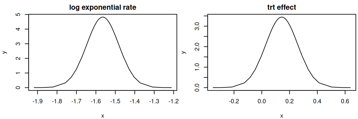
The results show the computation time followed by parameters estimates, the first one (i.e., Intercept) corresponds to the logarithm of the rate parameter for the exponential baseline hazard while the second one is our trt effect \(\gamma\). As we can see, this treatment effect matches well with the true value (i.e., 0.2). For the rate of the exponential, we can exponentiate it to compare with the true value (0.2). The summary of fixed effects is available in the summary.fixed argument of the fitted object:
exp(M_exp_inla$summary.fixed$mean[1])
[1] 0.2091438
We may however be interested in the uncertainty around this value which we only have on the log scale in R-INLA’s output. The function inla.tmarginal allows to transform posterior marginals with any function while the function inla.zmarginal can compute summary statistics over the transformed marginals. The posterior marginal distributions in an R-INLA fitted model are available directly in the fitted object as the marginals.fixed argument:
str(M_exp_inla$marginals.fixed)
List of 2
 $ (Intercept): num [1:43, 1:2] -1.92 -1.87 -1.82 -1.76 -1.73 ...
  ..- attr(*, "dimnames")=List of 2
  .. ..$ : NULL
  .. ..$ : chr [1:2] "x" "y"
 $ trt        : num [1:43, 1:2] -0.3504 -0.2872 -0.2143 -0.1258 -0.0834 ...
  ..- attr(*, "dimnames")=List of 2
  .. ..$ : NULL
  .. ..$ : chr [1:2] "x" "y"
par(mfrow=c(1,2), mar =c(4,4,2,0.3), cex=0.6)plot(M_exp_inla$marginals.fixed[[1]],type="l",main="log exponential rate")plot(M_exp_inla$marginals.fixed[[2]],type="l",main="trt effect")
Figure 2.1: Posterior marginal distributions from an R-INLA model fit. The left plot shows the posterior for the log exponential rate, and the right plot shows the posterior for the log-hazard ratio of the treatment effect.
And we can look at the transformed exponential rate as well as the hazard ratio of trt (instead of the log-hazard ratio as provided in R-INLA’s output) as shown in Figure 2.2:
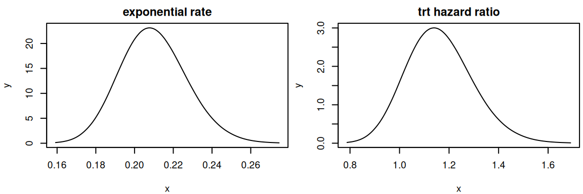
par(mfrow=c(1,2), mar =c(4,4,2,0.3), cex=0.6)Exp_rate_marg <-inla.tmarginal(exp, M_exp_inla$marginals.fixed[[1]])inla.zmarginal(Exp_rate_marg)
Figure 2.2: Posterior marginal distributions of the exponential rate and treatment hazard ratio. These plots show the posteriors from the R-INLA fit, transformed to their natural scales for easier interpretation.
The hazard ratio is easier to interpret and thus often favored as it directly multiplies the reference risk. In this example we could interpret as follows: The risk of event for individuals with trt=1 is increased by 16% on average compared to individuals with trt=0 with a 95% credible interval giving uncertainty between -8% and 45%.
We can fit the same model with INLAjoint, although the syntax is similar, the output is simplified:
Here the argument formSurv is the formula for the time-to-event outcome, with the response given as an inla.surv() object while dataSurv is the dataset that must contain the variables given in the formula. These two arguments are different from the usual formula and data to avoid confusion since INLAjoint can also deal with longitudinal models simultaneously. The argument basRisk gives the baseline hazard of event. Here we define the parametric exponentialsurv but other options are discussed in following sections.
The summary of the model directly gives the rate of the exponential baseline hazard and the log hazard ratio of treatment effect. To get the hazard ratio of treatment effect, the argument hr can be switched to TRUE in the call of the summary function:
Another difference with R-INLA’s raw output is the automatic computation of two goodness of fit criteria that can be used for model selection: the Deviance Information Criterion (DIC, Spiegelhalter et al. (2002)) and the Widely Applicable Bayesian Information Criterion (WAIC, Watanabe (2013)), available as:
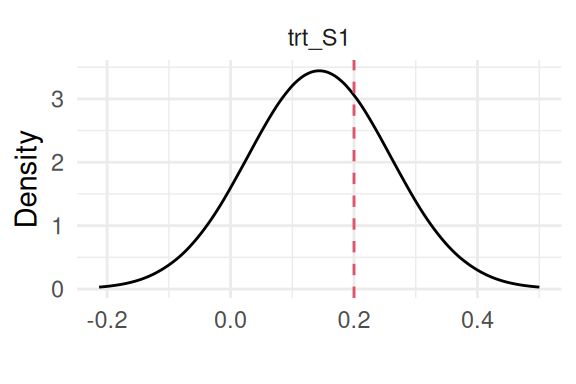
We can plot the fitted model directly with plot(M_exp) (see Section 1.5.4) to get the posterior marginals of all model parameters and the baseline hazard (Figure 2.3, Figure 2.4, Figure 2.5). INLAjoint uses the ggplot2 library for these plots (Wickham (2016)):
library(ggplot2)plot(M_exp)
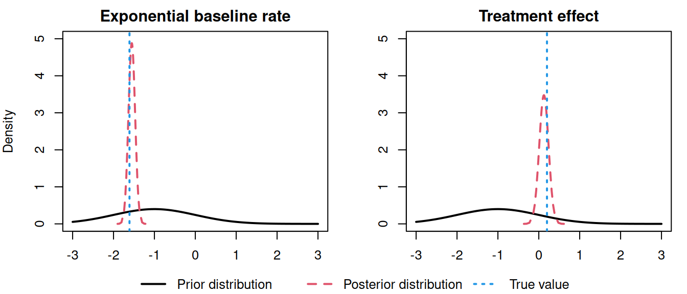
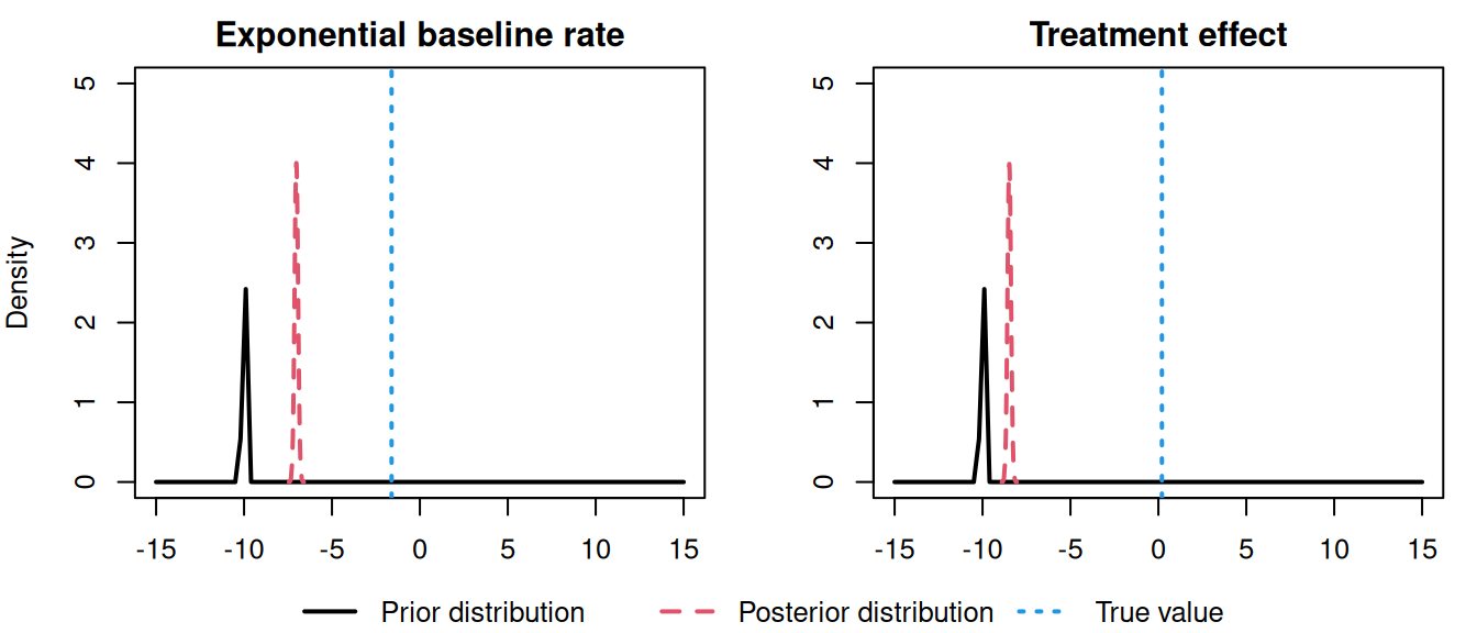
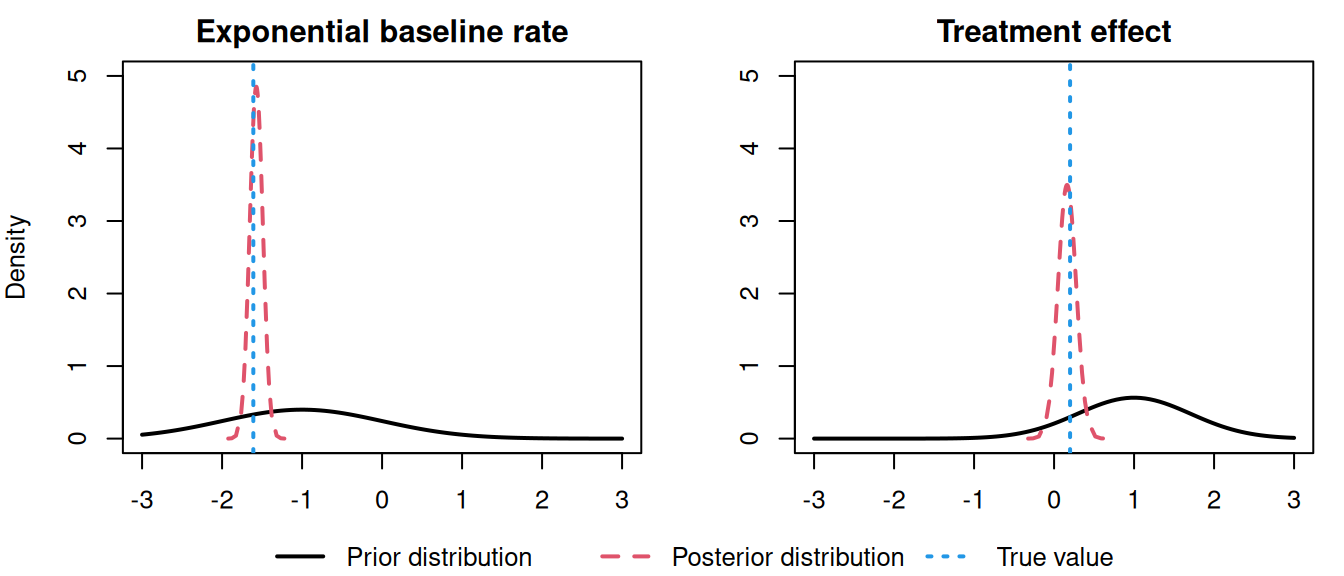
Figure 2.3: Posterior marginal distribution of the treatment effect (\(\gamma\)) from an exponential baseline hazard model. The dashed red line indicates the true value (0.2) used for data generation.
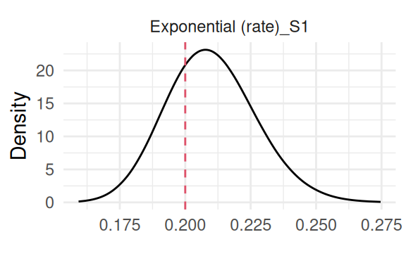
Figure 2.4: Posterior marginal distribution of the rate parameter (\(\mu\)) from an exponential baseline hazard model. The dashed red line indicates the true value (0.2) used for data generation.
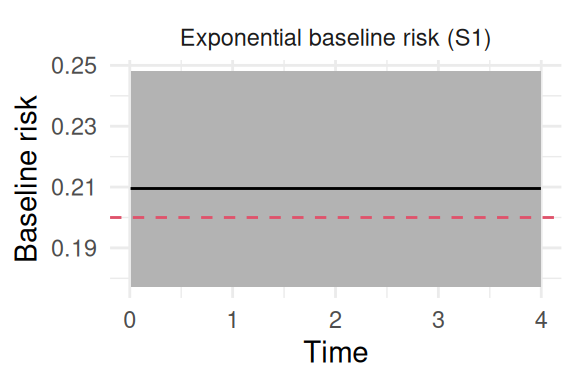
Figure 2.5: Posterior estimate of the exponential baseline hazard function. The solid black line shows the posterior mean, the shaded region represents the 95% credible interval, and the dashed red line indicates the true constant value (0.2) used for data generation.
Here we can see the model is able to find the true value of all the parameters, where the last plot shows the baseline hazard function over time (which is constant by definition here).
2.2.2 Weibull parametric baseline hazard & accelerated failure time model
The exponential baseline hazard is based on the often too simplistic assumption that the risk remains constant over time. We can add flexibility by allowing the risk to increase or decrease over time with the Weibull parametric distribution. This distribution has an additional shape parameter that controls the evolution of the baseline hazard over time, when shape>1, the hazard increases over time while it decreases when shape<1. When shape=1 the model reduces to the exponential and the baseline hazard is constant over time, the scale parameter then corresponds to the exponential rate.
With R-INLA, the Weibull likelihood has 2 variants which are fitting the same model but with different parametrizations (see inla.doc("weibull") for more details). The default variant in INLAjoint is variant 0, i.e., assuming the following definition of the hazard function:
\[\lambda_0(t) = \alpha \cdot t^{\alpha-1} \cdot \mu \cdot \exp(-\mu \cdot t^\alpha), \ \ \ \ \alpha>0, \ \ \ \ \ \mu>0 \] while variant 1 is defined as :
These two parametrizations are mathematically equivalent formulations of the same underlying Weibull model based on a transformation of the \(\mu\) parameter and their survival functions become identical under the transformation \(\mu_0=\mu_1^\alpha\).
Each variant’s structure aligns naturally with one of the two primary modeling frameworks in survival analysis, i.e., variant=0 is structured as a natural Proportional Hazards model, where covariates act multiplicatively on the baseline hazard. In contrast, variant=1 is structured as a natural Accelerated Failure Time (AFT) model, where covariates act to accelerate or decelerate the event timescale.
The Weibull distribution is unique in being the only commonly used distribution that belongs to both the PH and AFT model families. This means a single fitted model can be interpreted in two ways, and the parameters from one framework can be transformed into the other. We demonstrate this equivalence in the following.
We can start by fitting this model with INLAjoint, using the default variant 0, by just switching the basRisk argument to weibullsurv:
The key advantage of the Weibull model over the exponential model is the inclusion of the shape parameter \(\alpha\), which provides insight into the evolution of the hazard over time.
Again, the plot function can be used to display all posterior marginals and the baseline hazard evolution over time. Specific plots can be directly called by their name, for example for the baseline hazard:
plot(M_wei)$Baseline
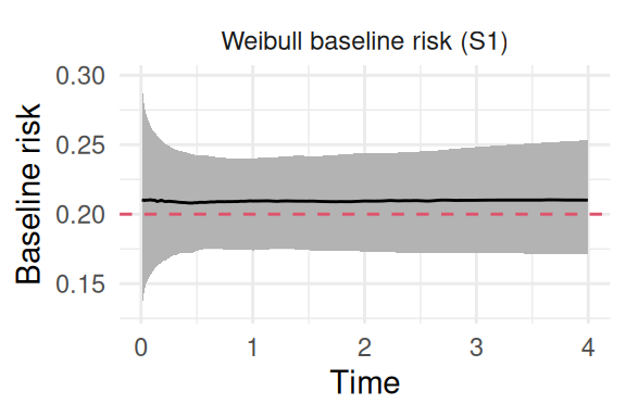
Figure 2.6: Posterior estimate of the baseline hazard from a Weibull model fitted to data with a true constant hazard. The solid black line is the posterior mean, the shaded region is the 95% credible interval, and the dashed red line indicates the true constant rate (0.2) used to generate data observations.
The posterior distribution for the shape parameter includes 1 in its 95% credible interval, meaning that the exponential baseline hazards is a reasonable assumption (it is indeed the true model we simulated from!). We can simulate data where the baseline hazard evolves over time (i.e., Weibull baseline), using the same method as for the exponential baseline hazard. The survival function for the current example is \(S(t) = \exp(-\mu\cdot t^\alpha \cdot\exp(\gamma \cdot trt_i))\). To simulate an event time \(t\), we again set a uniform random variable \(u \sim U(0,1)\) equal to the survival probability and solve for t: \[\log(u) = -\mu\cdot t^\alpha\exp(\gamma \cdot trt_i)\] Now we can rearrange the terms to isolate \(t\): \[t = \left(\frac{-\log(u)}{\mu\cdot \exp(\gamma \cdot trt_i)}\right)^{1/\alpha}\] This allows to simulate event times \(t\) based on uniform random numbers, the scale (\(\mu\)), the shape (\(\alpha\)) and regression parameters such as treatment effect (\(\gamma\)):
n=1000# number of individualsgamma=-1# treatment effectbaseScale=0.2# baseline hazard scalebaseShape=1.3# baseline hazard shapefollowup=4# study durationtrt <-rbinom(n, 1, 0.5) # trt covariateu <-runif(n) # uniform distribution for survival times generationeventTimes <-pmin((-(log(u))/(baseScale*exp(trt*gamma)))^(1/baseShape), followup)eventIndic <-as.numeric(eventTimes<followup) # event indicatordatWei <-data.frame(eventTimes, eventIndic, trt) # datasetsummary(datWei)
   eventTimes        eventIndic         trt
 Min.   :0.04007   Min.   :0.000   Min.   :0.00
 1st Qu.:1.68252   1st Qu.:0.000   1st Qu.:0.00
 Median :3.70431   Median :1.000   Median :0.00
 Mean   :2.90042   Mean   :0.535   Mean   :0.48
 3rd Qu.:4.00000   3rd Qu.:1.000   3rd Qu.:1.00
 Max.   :4.00000   Max.   :1.000   Max.   :1.00
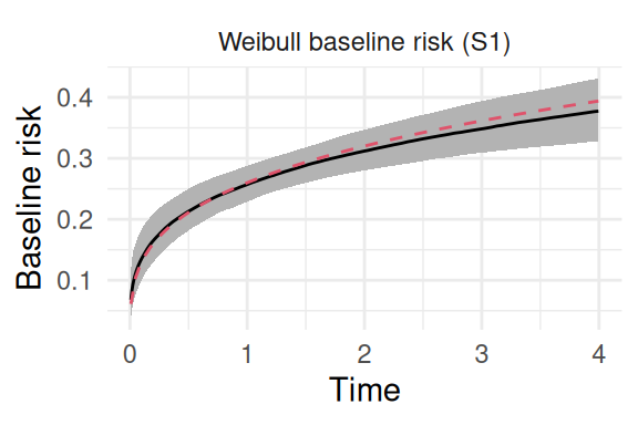
Now the shape parameter is set to 1.3, so that the baseline hazard increases over time. We can fit the model and plot it as in Figure 2.7:
Figure 2.7: Posterior estimate of the baseline hazard from a Weibull model fitted to data with a true increasing hazard. The solid black line is the posterior mean, the shaded region is the 95% credible interval, and the dashed red line represents the true Weibull hazard function used for data generation.
It is possible to switch variant in the control options of INLAjoint:
The results are slightly different but the underlying model is similar, one can match these results with basic transformations as shown below.
Another important point is the equivalence between the proportional hazards and the accelerated failure time model with the Weibull baseline hazard. Regardless of the variant, we can picture the model as PH or AFT as illustrated below (and compared with standard software for PH (R package eha, Broström (2022)) and AFT (R package survival, Terry M. Therneau & Patricia M. Grambsch (2000))):
We can see that both Weibull variants can be pictured as proportional hazards or accelerated failure time models, after some transformations of the posterior marginals. Of note, the Gompertz distribution is also an option in INLAjoint, although not presented here to avoid redundancies. However, an illustration of the defective Gompertz approach is presented in Section 2.7.2, which is an extension of the standard Gompertz distribution for baseline hazard to model data with a cure fraction.
There are several ways to define the baseline hazard function \(\lambda_0(t)\). In a parametric proportional hazards model, the baseline is defined as a specific function of time and additional parameters, the most common choices are the exponential, Weibull and Gompertz distributions. Piecewise constant functions do not make specific shape assumptions for the baseline hazard risk function, but tend to lack flexibility because of the assumption of piecewise constant hazards (and therefore “brutal” jumps in the hazard) with the risk of overfitting if too many intervals are defined. Additional flexible parametric methods (e.g., splines) have been proposed for the approximation of the baseline distribution function (Royston & Parmar (2002)).
Spline functions should be used with caution as their flexibility relies on an appropriate choice of the number of knots. They might overfit the data and provide a rough (i.e., not smooth) hazard function, which is usually not suitable as the risk function in the population of interest is usually expected to be smooth. For example Rondeau et al. (2007) uses penalization of the second-order derivatives of the splines, in order to prevent abrupt changes in the baseline hazard. Choosing the smoothing parameter is the difficult part of this method and can be done by approximate cross-validation techniques. Another approach uses random walks of order 1 or 2 (sometimes referred to as “Bayesian smooth splines”), this approach is flexible and requires only a single parameter (the precision of the random walk) since the baseline hazard then relies on the data with a smoothness constraint (Alvares et al. (2024)). It has been shown to outperform traditional splines approximation in terms of accuracy (Rustand et al. (2023)) and converges to a stable shape when the number of knots is increased.
Alternatively, leaving the baseline hazard completely unspecified is possible when the partial likelihood technique is applied but the estimation of the standard errors of the regression parameters is computationally intensive (especially for joint models) and prediction of survival probabilities is cumbersome (Xu et al. (2020)).
The baseline hazard is not observed directly and we may not know its expected shape. If it is not monotonic, the parametric approaches described above will fail to capture it properly, which is why the Cox model is often preferred as it makes no assumption on the shape of the baseline.
It has been shown that the full likelihood of a Cox model can be approximated with that of a Poisson regression by Holford (1976), Whitehead (1980) and Johansen (1983). The key idea is to convert the continuous-time hazard function into a discrete-time event count. If the time intervals are small enough, the hazard can be considered roughly constant within each interval. Then, the number of events in each interval follows a Poisson distribution, where the mean is proportional to the hazard in that interval.
The Poisson approximation in discrete time is based on the assumption that the number of events \(N_i\) in a small time interval of length \(\Delta t\) follows a Poisson distribution: \[N_i|\mu_i \sim \textrm{Poisson}(\mu_i)\] where the mean \(\mu_i\) is proportional to the hazard within the interval such that: \[\mu_i = \lambda_i\left(t\right) \Delta t.\] This approximation becomes more accurate as the time intervals become shorter. However, it’s important to note that this approximation may introduce error if the hazard changes rapidly within the intervals but if each unique event time is made into its own interval the partial likelihood approach for the Cox model can be replicated exactly. This is the method used to fit the Cox proportional hazards model with INLA.
In practice, we use an offset term to match exactly the event time and censoring time when they occur within an interval. Moreover, since more intervals involve a more flexible approximation of the baseline, INLAjoint uses random walk priors instead of piecewise constant approximation to avoid overfitting and ensure a smooth baseline hazard function. The Poisson regression model then fits with the LGM framework described in Chapter 1, and can be fitted with INLA.
In order to see how this “Poisson trick” works with R-INLA, we first need to decompose the follow-up into intervals. This is done with the inla.coxph function. Note that with INLAjoint, this step is done internally as illustrated later in this section (we show in details how this is done with R-INLA for transparency and a better understanding of how INLAjoint works).
There are now 10 lines in the expanded dataset for individual 1 where each line corresponds to an interval of the follow-up. For example the third line corresponds to an interval of size 0.27 (column E..coxph) that starts at time 0.53 (column baseline.hazard) without observing the event (column y..coxph). The last line is a smaller interval as it stops at the event time.
The cutpoints are defined automatically as equidistant between 0 and the maximum observed follow-up time. We can see the cutpoints in the object created:
Expanded_data$data.list # cutpointsseq(0, max(datWei$eventTimes), len=16) # default is equidistant
The default number of intervals is 15 but it can be changed in control.hazard when creating the expanded dataset, by setting the argument n.intervals (see ?control.hazard for more details on available arguments). It is also possible to manually setup these cutpoints with the argument cutpoints (which then overwrites the argument n.intervals). Finally the argument model allows to choose between random walk of order one (model = "rw1") and order two (model = "rw2").
We can then fit the model with R-INLA:
datRW <-append(Expanded_data$data.list, Expanded_data$data)M_INLA_rw1 <-inla(Expanded_data$formula, data = datRW,E=Expanded_data$E, family = Expanded_data$family)summary(M_INLA_rw1)
Time used:
    Pre = 0.217, Running = 0.279, Post = 0.0323, Total = 0.528
Fixed effects:
              mean    sd 0.025quant 0.5quant 0.975quant   mode kld
(Intercept) -1.236 0.055     -1.343   -1.236     -1.129 -1.236   0
trt         -0.982 0.094     -1.165   -0.982     -0.798 -0.982   0

Random effects:
  Name    Model
    baseline.hazard RW1 model

Model hyperparameters:
                               mean    sd 0.025quant 0.5quant 0.975quant  mode
Precision for baseline.hazard 30.97 41.33       4.48    20.09     119.12 10.49

Marginal log-Likelihood:  -2641.08
 is computed
Posterior summaries for the linear predictor and the fitted values are computed
(Posterior marginals needs also 'control.compute=list(return.marginals.predictor=TRUE)')
The results include two fixed effects, where the intercept corresponds to the average log-baseline hazard and deviations from this average are captured by the random walk (i.e., the random walk has a sum-to-zero constraint). It is also possible to remove this constraint in the control.hazard arguments, then the average of the random walk replaces this intercept (this is the strategy used in INLAjoint). The precision of the random walk (i.e., inverse of the variance) is given as an hyperparameter, the lower the value, the higher the deviations from the average baseline hazard. Note that this model can also be replicated in R-INLA with the coxph likelihood, although this approach is limited to the standard Cox PH. In the following, we show how to replicate this model with INLAjoint which facilitates the use of INLA for such models.
We start by defining the random walk of order one proportional hazards model:
The summary shows the variance of the random walk and the log hazard ratio of treatment effect. As illustrated for parametric proportional hazards model, we can directly plot the baseline hazards with the plot function, as shown in Figure 2.8:
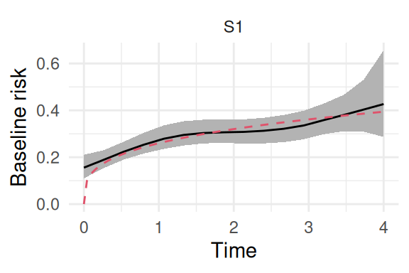
plot(M_rw1)$Baseline
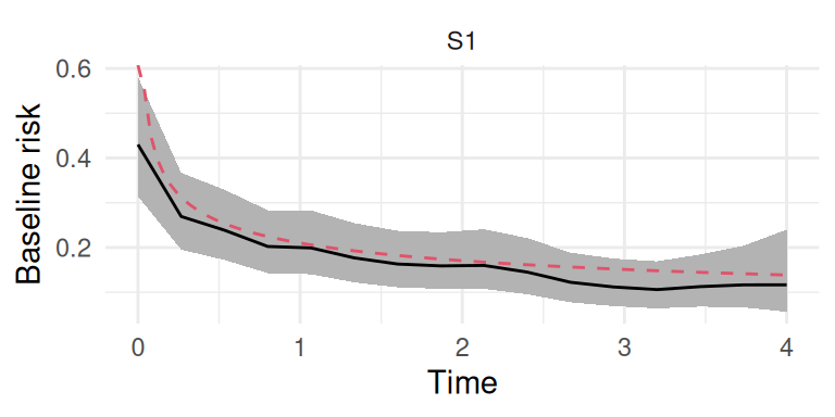
Figure 2.8: Posterior estimate of the baseline hazard function using a random walk of order 1. The solid black line is the posterior mean, the shaded region is the 95% credible interval, and the dashed red line is the true underlying Weibull hazard function.
We can also fit the random walk of order two, which is smoother due to the smoothness constraint relying on the second order closest neighbors:
Figure 2.9: Posterior estimate of the baseline hazard function using a random walk of order 2. The solid black line is the posterior mean, the shaded region is the 95% credible interval, and the dashed red line is the true underlying Weibull hazard function.
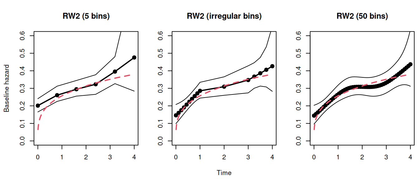
An important point is the number of intervals to decompose the follow-up, the default for both random walk methods is 15 equidistant bins but increasing the number of bins will get us closer to the stochastic model and does not lead to overfitting as observed with commonly used splines (Van Niekerk et al. (2023)). We can compare the impact of the number and position of bins. First we fit a model with 5 intervals, this is set with the argument NbasRisk:
Still nearly identical, meaning that the baseline hazard is well approximated, even with a few intervals. This may not be true for more complex examples with important changes in the trend of the baseline hazard. We can set manually the position of the bins with the argument cutpoints, here for example we include many points in the early/late follow-up:
Figure 2.10: Comparison of RW2 baseline hazard estimates under different interval specifications. Each plot shows the posterior mean (points and line) and 95% credible interval for the baseline hazard estimated with: 5 equidistant bins (left), irregularly spaced bins (middle), and 50 equidistant bins (right). The true Weibull hazard is the dashed red line.
We can see how the number and position of the bins control the flexibility of the approximation, without any cost of having “too many” bins, unless for the increased computation time. The choice of the number of bins therefore involves a trade-off between flexibility and computational cost. For smoothly varying hazards, the default value of NbasRisk (15 intervals) is often sufficient. For studies with long follow-up or where the hazard is expected to be highly dynamic, increasing this value can provide greater flexibility. As demonstrated, the random walk prior provides strong regularization against overfitting, making the model robust to a large number of intervals.
A sensitivity analysis is always a recommended practice to ensure the results are stable. Beyond the random walks, it is technically possible to define any function for the baseline hazards and while this book focuses on the currently available options, new options could be developed if needed.
2.2.4 Illustrative example
To make the theoretical distinctions between parametric and semi-parametric baseline hazard models more concrete, we now apply these approaches to a real-world dataset. This practical illustration relies on the clinical trial data for primary biliary cholangitis (pbc2 dataset), which was previously introduced in Chapter 1. The objective is to visually compare the posterior estimates of the baseline hazard function under four distinct sets of assumptions: the constant hazard of the Exponential model, the monotonically constrained hazard of the Weibull model, and the flexible, smooth hazards estimated using first-order (RW1) and second-order (RW2) random walks.
This comparison will serve to highlight the strengths and limitations of each approach, demonstrating how model flexibility interacts with data and how restrictive assumptions can influence the resulting inference about the underlying event risk.
We first load and prepare the pbc2 dataset, extracting the relevant time-to-event data for the analysis (we consider the hazard of transplantation as a function of drug). Subsequently, we fit the four distinct survival models, each defined by a different assumption for the baseline hazard. Then, we can extract the posterior mean and 95% credible intervals for the baseline hazard from each model and plot these estimates for a direct visual comparison.
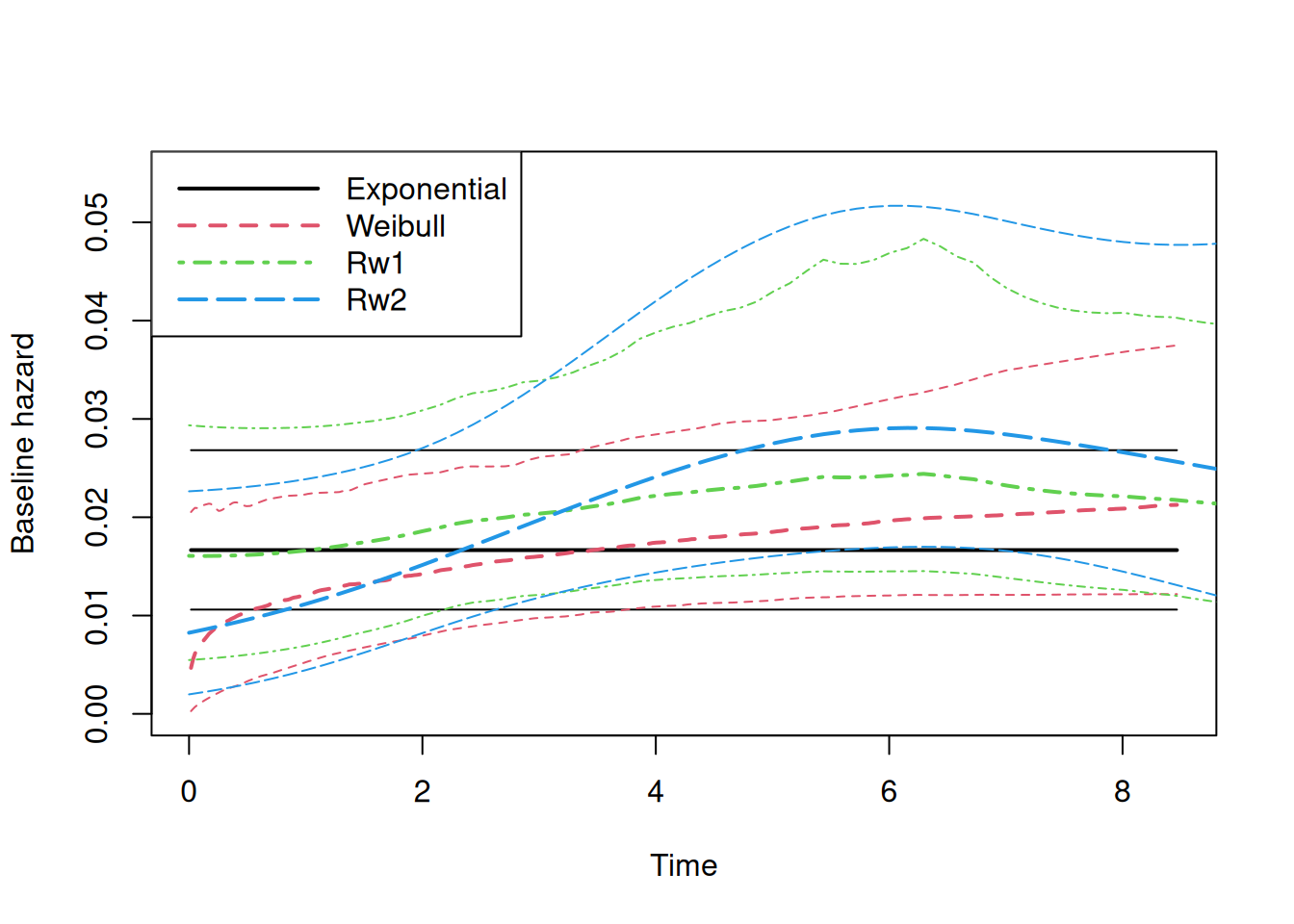
Figure 2.11: Comparison of estimated baseline hazard functions for the PBC dataset. The plot shows the posterior mean and 95% credible interval of the baseline hazard from four models: Exponential (black solid line), Weibull (red dashed line), RW1 (green dotted-dashed line), and RW2 (blue long-dashed line).
The exponential model provides a constant hazard that represents a reasonable average risk over the follow-up period but fails to capture the temporal dynamics of the event risk. The Weibull model, with its added flexibility, captures an initial increase in the baseline hazard, aligning well with the random walk estimates during the first two years where the density of observed events is highest. However, its rigid parametric assumption of monotonicity forces it to overlook the subsequent change in trend, where a plateau and potential decrease is suggested by the more flexible random walk models. This difference highlights how parametric assumptions can introduce bias, particularly when the true hazard shape is non-monotonic.
The random walk models, by contrast, are sufficiently flexible to adapt to the data across the entire follow-up. They not only capture the initial increase in risk but also the subsequent stabilization, a pattern that may reflect important underlying changes in the disease’s natural history. The models largely agree where the data is most informative (early follow-up), and diverge where it is sparse (late follow-up).
This comparison has profound implications for predictions, particularly for the extrapolation beyond the observed range of the data. The random walk models, being inherently data-driven and non-parametric in nature, are not naturally defined beyond the maximum observation time. Their predictive mechanism defaults to a simple linear projection of the last observed trend. Conversely, parametric models like the Weibull are mathematically defined for any time point \(t>0\), making them an appealing choice for extrapolation.
However, this should be used with caution. The ability of a parametric function to produce a value does not confer validity upon it. Extrapolating a functional form that already shows clear signs of misspecification within the observed data range (as the Weibull model does here) is tricky and can lead to biased results and misleading conclusions. The apparent certainty of the parametric extrapolation is an illusion if the underlying assumption is incorrect. Therefore, while parametric assumptions can be useful for interpolation and short-term prediction, we warn against extrapolating model predictions far beyond the temporal support of the data. Such predictions are not data-driven inferences but are instead pure assumptions about future behavior that cannot be validated by the data at hand.
2.3 Inference and prediction of hazard and survival functions
We may be interested in the computation of survival probabilities and survival curves for some scenarios from a fitted survival model (see Section 1.5.5). For example, let’s compute survival probabilities based on the random walk of order 2 model fitted in Section 2.2.3, conditional on the covariate trt. In order to do so, we first create a new dataset that describes our scenarios of interest. This dataset must match the dataset structure as used to fit the model we want to predict from, meaning that all covariates included in the model should be in this new dataset (2 scenarios here means 2 lines). Since we are only interested in trt = 0 vs. trt = 1. We can use the column trt to identify the scenario through the argument id. For more complex scenarios (multiple specific values of a non-binary covariate or multiple covariates), an additional column is needed to identify each scenario (i.e., with an unique value for each scenario).
NewData <-data.frame("trt"=0:1);NewData
  trt
1   0
2   1
Then we call the predict function:
P <-predict(M_rw2, NewData, horizon =4, id="trt")
The first argument is the model from which we derive predictions, the second argument is the new dataset that gives the scenarios of interest (i.e., here we want to compute the hazard function for trt=0 and trt=1). The argument horizon gives the time until which we want to compute the predictions and the argument id gives the column name for scenarios. See Section 1.5.5 for more details about how predictions are computed with INLAjoint.
The object P contains the results of the predictions, it is a list of 2 items, “predL” for prediction of longitudinal outcomes (see Chapter 3) and “predS” for predictions of survival outcomes. A data frame contains the result of the predictions with the first column identifying the scenario, eventTimes for the time at which the hazard function is computed, Outcome to identify the outcome when a multi-outcome model is used and the rest are summary statistics of the corresponding hazard function. The time points are defined automatically as 50 equidistant points between 0 and horizon. It is possible to modify the number of time points with the argument NtimePoints. Moreover, one can directly give a vector of time points to predict the risk at these points specifically with the argument timePoints.
Now we’re interested in the survival function, we can compute it by setting the argument survival=TRUE in the call of the predict function:
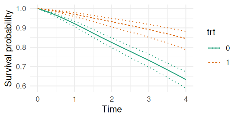
P <-predict(M_rw2, NewData, horizon =4, id="trt", survival=TRUE)str(P)
Figure 2.12: Predicted survival probabilities conditional on treatment group. The plot shows the estimated survival curves for the treatment group (trt=1, orange dashed line) and the control group (trt=0, green solid line). Dotted lines form the 95% credible intervals.
Note that for survival functions, the integration of the hazard function is based on the decomposition of time with timePoints, it is therefore important to have enough time points between the entry in the at-risk period and the horizon to get accurate estimates of the survival function.
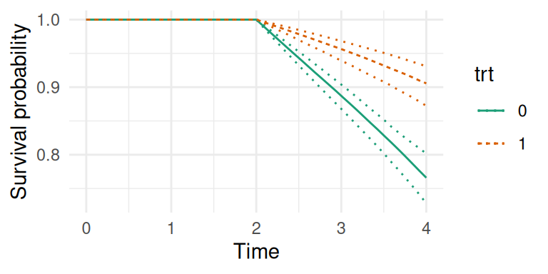
Here the entry in the at-risk period is time 0 but this can be modified with the argument Csurv, for example we can assume the at-risk period starts at time 2:
Figure 2.13: Predicted survival probabilities conditional on being event-free at time 2. The survival probabilities are calculated starting from time 2, as specified by the Csurv=2 argument.
2.4 Time-dependent covariates
It is possible to include time-dependent covariates in a survival model, they can be classified into two categories:
Exogeneous (or external) covariates remain measurable and their distribution is unchanged after the occurrence of the event.
Endogeneous (or internal) covariates’ distribution is affected by the event.
The proportional hazards model can handle exogeneous time-dependent covariates but the likelihood requires knowing the value of these covariates for all subjects at risk over the follow-up while covariates are often only measured at some occasions, therefore requiring to impute values. Most biomarkers of interest in clinical research are endogeneous variables, their values are affected by a change in the risk of occurrence of the event. For example in a cancer clinical trial, if a treatment reduces both the risk of death and the size of tumors, adjusting a survival model on the size of tumors may severely bias the effect of treatment on the risk of death (because some of the treatment effect will be captured by tumor size).
It is often of interest to estimate the effect of the treatment on the biomarker. The biomarker may be censored by the event and its value is only known at the specific time points at which it is measured. Separate models for the longitudinal and survival outcomes are prone to bias when the two outcomes are associated (Rubin (1976), Wang & Taylor (2001)). Alternatively, two-stage models can fit a longitudinal model and subsequently use the estimated longitudinal trajectory of the biomarker as a covariate in the survival model (Tsiatis et al. (1995)). They account for measurement error of the biomarker in the survival model but fail to account for informative drop-out in the longitudinal model. Ignoring informative censoring in a longitudinal analysis can lead to biased covariates’ effect estimates (Garcı́a-Hernandez et al. (2020)).
In contrast, joint models offer the advantage of dealing with informative drop-out, measurement error and missing biomarker measurements not at random in the longitudinal and survival regression models (Ibrahim et al. (2010)). Being able to handle time-dependent covariates in survival models is necessary to fit most joint models (see Chapter 4).
With INLA, one can take advantage of the decomposition of the follow-up into intervals in order to account for time-varying covariates. These intervals can be arbitrary small without changing the likelihood of the model as we can reconstruct the follow-up with left truncation and right censoring. Let’s illustrate this with an example based on simulated data from Section 2.2.2. We consider the Weibull parametric baseline hazard but the same applies to other baseline hazard options. The standard model will assume each data point has an unique contribution to the likelihood (as described in Section 2.2.2):
# 1 observation per individualM_weib_1 <-inla(inla.surv(eventTimes, eventIndic) ~ trt,data=datWei, family ="weibullsurv")round(rbind(M_weib_1$summary.fixed[,1:2], M_weib_1$summary.hyperpar[,1:2]),4)
                                   mean     sd
(Intercept)                     -1.6067 0.0779
trt                             -0.9884 0.0933
alpha parameter for weibullsurv  1.2811 0.0505
length(M_weib_1$.args$data[[1]]) # original data size
[1] 1000
We can decompose the follow-up with 15 intervals of the same length between time 0 and the maximum follow-up time:
This decomposition is similar to the decomposition used for the baseline hazard with random walk to replicate the Cox model introduced in Section 2.2.3. We can therefore use the same function to set it up:
Both data contain the same amount of information, the first basically means “Individual 1 was observed for 2.43 units of time until he observed the event” while the second decomposes into “Individual 1 was observed for 0.27 units of time without observing the event” followed by “Individual 1 was observed between time 0.27 and 0.53 without observing the event”, …, “Individual 1 was observed between time 2.40 and 2.43 until the event was observed”. Since the amount of data information that contributes to the likelihood is the same between these two data formats, we can compare the results (note the use of truncation in inla.surv to be able to start the follow-up from where it stopped in the expanded format):
                                   mean     sd
(Intercept)                     -1.6067 0.0779
trt                             -0.9884 0.0933
alpha parameter for weibullsurv  1.2811 0.0505
# data size after decomposition into 15 intervalsprint(paste0("N = ", length(Itv$data[[1]])))
[1] "N = 11140"
The results are identical but in the second format, we can now include a covariate with values specific to each interval. The number of intervals can be arbitrarily large to capture smooth evolution of covariates over time. We can do the same decomposition with 100 cutpoints:
                                   mean     sd
(Intercept)                     -1.6067 0.0779
trt                             -0.9884 0.0933
alpha parameter for weibullsurv  1.2811 0.0505
# data size after decomposition into 100 intervalsprint(paste0("N = ", length(Itv2$data[[1]])))
[1] "N = 72783"
One can now clearly see how this allows to include time-dependent covariates by adding the covariate of interest in this data format where the value can differ for each interval. Moreover, it is possible to match the decomposition of the follow-up into intervals with measurement occasions of the time-dependent covariate to assume an (often unrealistic) constant value between measurement occasions to avoid imputation. This is done with the argument cutpoints.
2.5 Interval censoring
Interval censoring occurs when the exact time of an event is unknown but is known to fall within a specific time window (e.g., between two clinic visits or lab tests). Unlike right-censoring (where an event is only known not to have occurred by the last observation), interval censoring arises when events are detected at intermittent measurements.
Interval censoring is available with parametric baseline hazard functions but requires additional steps with random walks as the integral over the interval is not straightforward and needs sampling to be taken into account properly (see for example Pan (2000)).
We can simulate interval censored data with the R package iCenReg (Anderson-Bergman (2017)), and then estimate the model with INLAjoint:
library(icenReg) # for data simulation# Simulate data from a ph model where covariates # x1 and x2 have effect b1 and b2, respectively.sim_data <-simIC_weib(n =5000, b1 =0.5, b2 =-0.5)sim_data$ev <-ifelse(sim_data$u==Inf, 0, 3)M_intcen <-joint(inla.surv(time=l, time2=u, event=ev) ~ x1 + x2, dataSurv = sim_data, basRisk="weibullsurv")summary(M_intcen)
The true values of the two covariates effect x1 and x2 (0.5 and -0.5, respectively) are well recovered by the model. In this example, we can see how interval censoring is handled through the specification of the arguments time and time2 that corresponds to the left and right bounds of the interval, respectively. The event indicator is set to 3 which means interval censored observation. It is possible to have a combination of interval censored observations and observed events (event=1) as well as right censored observations (event=0). More examples are available in Van Niekerk & Rue (2022).
2.6 Stratified proportional hazards model
Sometimes the baseline hazard may differ across subgroups but the relative effect of covariates remains identical within each stratum, in this case one can use the stratified proportional hazards model which allows for greater flexibility by accounting for heterogeneity across distinct populations. We can simulate data where a binary covariate strata defines two subgroups with each a specific baseline hazard. For strata=0, the baseline hazard is defined as Weibull with a shape parameter equal to 1.5, meaning that the baseline hazard increases over time while for strata=1 the shape parameter is set to 0.7 so that the baseline hazard decreases over time:
n=1000# number of individualsgamma=-1# treatment effectbaseScale=0.5# baseline hazard scale strata 1baseShape=1.5# baseline hazard shape strata 1baseScale2=0.5# baseline hazard scale strata 2baseShape2=0.7# baseline hazard shape strata 2followup=4# study durationtrt <-rbinom(n, 1, 0.5) # trt covariatestrata <-as.integer(rbinom(n, 1, 0.5))+1u <-runif(n) # uniform distribution for survival times generationeventTimes <-ifelse(strata==1, (-(log(u))/(baseScale*exp(gamma*trt)))^(1/baseShape), (-(log(u))/(baseScale2*exp(gamma*trt)))^(1/baseShape2))eventIndic <-as.numeric(eventTimes<followup) # eventTimes indicatoreventTimes <-pmin(eventTimes, followup)datStr <-data.frame(eventTimes, eventIndic, strata, trt) # datasetsummary(datStr)
   eventTimes          eventIndic        strata           trt
 Min.   :0.0005999   Min.   :0.000   Min.   :1.000   Min.   :0.00
 1st Qu.:0.8365166   1st Qu.:0.000   1st Qu.:1.000   1st Qu.:0.00
 Median :1.9359808   Median :1.000   Median :2.000   Median :1.00
 Mean   :2.1874111   Mean   :0.718   Mean   :1.509   Mean   :0.52
 3rd Qu.:4.0000000   3rd Qu.:1.000   3rd Qu.:2.000   3rd Qu.:1.00
 Max.   :4.0000000   Max.   :1.000   Max.   :2.000   Max.   :1.00
We can fit a stratified proportional hazard model by setting the argument strata in control options. We can directly plot all stratum-specific baseline hazards curves with the plot function:
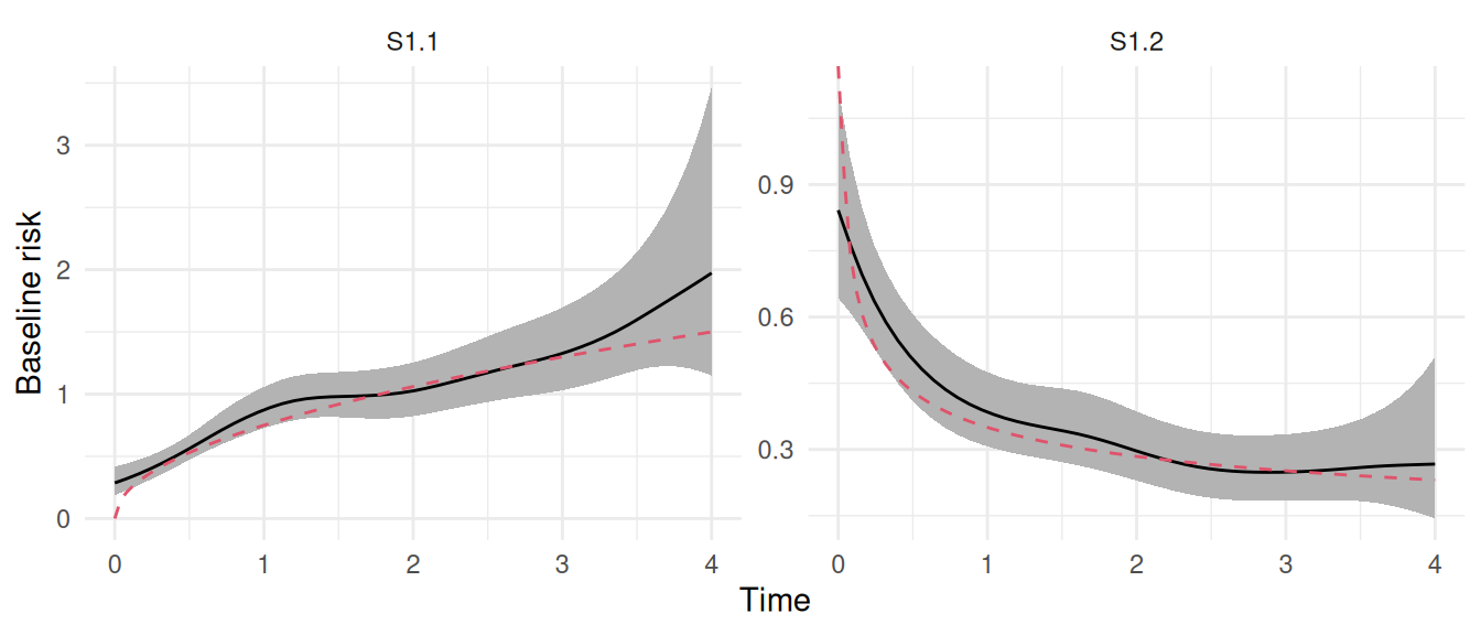
Figure 2.14: Estimated baseline hazard functions from a stratified proportional hazards model. The left plot (S1.1) and right plot (S1.2) show the distinct baseline hazards estimated for the two strata. In each plot, the solid line represents the posterior mean of the baseline hazard, and the shaded region is the 95% credible interval. The dashed red lines indicate true curves used to generate data observations. The plot demonstrates the model’s ability to capture different, flexible baseline hazard profiles for each stratum.
We can see that we captured properly the strata-specific baseline hazard functions with random walks sharing a common variance hyperparameter. We can verify the fixed effect of treatment in the summary:
The effect of treatment here is assumed to be the same for both strata and match with the true value used for simulations (-1).
2.7 Cure fraction models
2.7.1 Standard mixture cure model
The mixture cure model is used to analyze survival data with a cure fraction, meaning a proportion of the population is not at risk of experiencing the event of interest. In this framework, the population is conceptualized as a mixture of two distinct subgroups: “cured” individuals, who will never experience the event, and “uncured” individuals, who remain at risk. The survival function for the entire population is modeled as a weighted average of the survival functions of these two groups.
Let \(p(C=1)\) denote the probability of being cured and \(\lambda_{i}(t|C=0)\) the survival for the part of the population that is not cured, the mixture cure model is defined by:
\[\left\{
\begin{array}{ c @{{}{}} l @{{}{}} r }
\textrm{Logit}(p(C=1)) &= \beta_{0} + \beta_{1}\cdot X_{1i} + \beta_{2}\cdot X_{2i} & \text{(probability of being cured)} \\
\lambda_{i}(t|C=0)&=\lambda_{0}(t)\ \textrm{exp}\left(\gamma_1\cdot Z_{1i} + \gamma_2\cdot Z_{2i}\right) & \text{(survival for non-cured)}
\end{array}
\right.\]
The model includes a logistic regression model for the probability of being cured and a proportional hazards model for the time to event for the uncured individuals.
The cure fraction can be included in any survival model and can handle both right and interval censoring. However, only parametric baseline hazard can be defined at the moment for mixture cure models and the covariates that affect the probability of being cured can be associated to fixed effects only (i.e., no random effects in the logistic part). We can simulate data from this model with the R package mixcurelps (Gressani et al. (2022)):
# library(mixcurelps) # used to simulate data# since it causes install error on some OS, the following code replicates# the simulation code from mixcurelps without requiring the libraryn <-5000 ; W1=0.25 ; W2=1.45beta0=-0.70 ; beta1=1.15 ; beta2=-0.95 ; gamma1=-0.10 ; gamma2=0.25X <-cbind(1, rnorm(n), rbinom(n, 1, 0.5))B <-rbinom(n, 1, (1+exp(X %*%c(beta0, beta1, beta2)))^-1)Z <-cbind(rnorm(n), rbinom(n, 1, 0.4))Tlat <- (-log(runif(n)) / (W1 *exp(Z %*%c(gamma1, gamma2))))^(1/W2)Tlat[Tlat >8] <-8; Tlat[B ==0] <-20000; C <-pmin(rexp(n, 0.16), 11)tobs <-pmin(Tlat, C); delta <-as.numeric(Tlat <= C)simdat <-setNames(data.frame(tobs, delta, X, Z),c("tobs","event","Intercept","x1","x2","z1","z2"))M_mc <-joint(formSurv=inla.surv(tobs, event,cure=cbind("Int"=1, "x1"=x1, "x2"=x2)) ~ z1 + z2,basRisk ="weibullsurv", dataSurv=simdat)summary(M_mc)
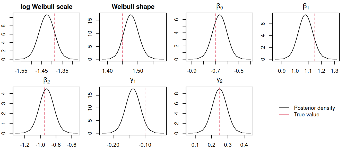
The argument cure in the definition of the outcome with inla.surv allows to define covariates that affect the probability of being cured. Here we set an intercept and the effect of the two covariates X1 and X2. Figure 2.15 shows the posterior density of all the model parameters:
Figure 2.15: Posterior marginal distributions for the parameters of a mixture cure model. The plots show posteriors for the Weibull parameters, cure probability fixed effects (\(\beta_0, \beta_1, \beta_2\)), and survival component fixed effects (\(\gamma_1, \gamma_2\)). Dashed red lines indicate true values.
With mixture cure models, we are often interested in the probability of being cured. Since we use a logistic regression model with a logit link, we need to apply the inverse logit function to the linear predictor to get probabilities. For example for the probability of being cured for the reference individual (i.e., X1 = X2 = 0):
inla.zmarginal(inla.tmarginal(function(x) 1/(1+exp(-x)),
               M_mc$marginals.hyperpar$`beta1 for Weibull-Cure`))
For the situations where X1 \(\neq\) 0 and/or X2 \(\neq\) 0, we can sample from the posterior distributions of the model and compute the corresponding linear combinations for each sample (it is also possible to setup linear combinations directly in R-INLA but this is not presented in this book).
# First sample values of intercept, X1 and X2's fixed effects# Note how for mixture cure, these fixed effects are considered as # hyperparameters for internal computations purposeS <-inla.hyperpar.sample(10^4, M_mc)[, 2:4]# Then we can compute the proba of being cured for different scenarioslist("X1 = 0, X2 = 0"=summary(1/(1+exp(-S[,1]))),"X1 = 0, X2 = 1"=summary(1/(1+exp(-rowSums(S[,c(1,3)])))),"X1 = -2, X2 = 1"=summary(1/(1+exp(-(S[,1]-2*S[,2]+S[,3])))))
$`X1 = 0, X2 = 0`
   Min. 1st Qu.  Median    Mean 3rd Qu.    Max.
 0.2869  0.3306  0.3401  0.3400  0.3492  0.3910

$`X1 = 0, X2 = 1`
   Min. 1st Qu.  Median    Mean 3rd Qu.    Max.
 0.1357  0.1627  0.1699  0.1703  0.1776  0.2160

$`X1 = -2, X2 = 1`
   Min. 1st Qu.  Median    Mean 3rd Qu.    Max.
0.01274 0.02081 0.02311 0.02337 0.02564 0.04149
Here we can see the different probabilities of being cured conditional on different combinations of covariates values.
2.7.2 Defective Gompertz distribution
While the mixture model offers an intuitive framework, it conceptualizes the population as two separate groups, requiring an additional logistic model for the cure probability. The defective Gompertz distribution provides a more parsimonious and integrated alternative. Instead of modeling a separate cure parameter, this approach includes the cure fraction directly into the survival function itself.
The defective Gompertz distribution reframes the cure fraction as an asymptotic property of the survival distribution. This unified framework can lead to more stable estimation, as traditional mixture models may suffer from convergence issues, particularly when the data suggest a large/low cure fraction. Moreover, the defective Gompertz distribution reduces to the standard Gompertz when there is no evidence for a cure fraction in the observed data (assuming the Gompertz distribution is flexible enough to capture the true hazard in the population). This allows to investigate the presence (or not) of a cure fraction in a population while the traditional cure fraction model fails to converge if there is no evidence for a cure fraction in the data (because the probability of being cured is 0, which corresponds to an infinite value in the scale of the logistic model). The Gompertz distribution is characterized by a hazard function that changes exponentially over time. Its probability density function is given by:
\[f(t) = \mu \cdot \exp(\alpha\cdot t) \exp\left(-\frac{\mu}{\alpha}(\exp(\alpha\cdot t)-1)\right)\] for \(t>0\), where \(\alpha\) is the shape parameter and \(\mu>0\) is the scale parameter. The corresponding survival function is: \[S(t) = \exp\left(-\frac{\mu}{\alpha}(\exp(\alpha\cdot t)-1)\right)\] The key to this approach lies in the shape parameter, \(\alpha\), which is not constrained to be positive in the defective formulation of the Gompertz distribution. When \(\alpha\) is negative, the hazard function decreases over time and approaches zero, causing the survival function to become defective (i.e., it does not converge to zero). Instead, it does reach a plateau at a value greater than zero, which represents the cure fraction.
The cure proportion, \(p\), is calculated as the limit of the survival function as \(t \rightarrow \infty\) when \(\alpha < 0\): \[p = \lim_{t\to\infty} S(t) = \exp\left(\frac{\mu}{\alpha}\right)\] This formula shows that the cure fraction is an intrinsic property derived directly from the distribution’s parameters, not an external parameter estimated separately. The parameter \(\alpha\) controls both the shape of the hazard curve and the existence of a cure fraction. If the credible interval over \(\alpha\) only includes negative values, the data support the presence of a cure fraction in the population.
We can simulate from this model, assuming a simple model including a cure fraction and a single fixed effect (trt):
   eventTimes         eventIndic         trt
 Min.   :0.002092   Min.   :0.000   Min.   :0.00
 1st Qu.:0.684837   1st Qu.:0.000   1st Qu.:0.00
 Median :2.170316   Median :0.000   Median :1.00
 Mean   :2.860677   Mean   :0.264   Mean   :0.52
 3rd Qu.:4.725078   3rd Qu.:1.000   3rd Qu.:1.00
 Max.   :7.805085   Max.   :1.000   Max.   :1.00
Fitting the model with INLAjoint is straightforward. We just need to specify the argument basRisk = "dgompertzsurv" to use the defective Gompertz likelihood for the survival submodel:
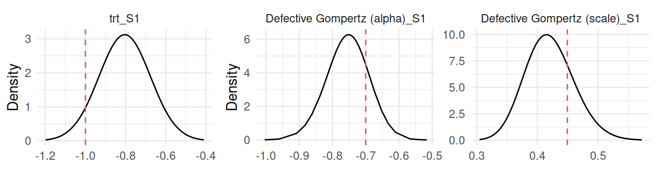
The model seems to successfully recover the true parameters used to generate the data, we can plot the posterior marginals of all the model parameters (Figure 2.16):
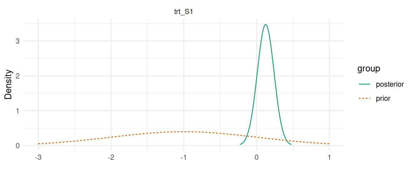
Figure 2.16: Posterior marginal distributions for the parameters of a defective Gompertz cure model. The plots display the posterior densities for the treatment effect (trt_S1), the defective parameter (Defective Gompertz (alpha)_S1), and the scale parameter (Defective Gompertz (scale)_S1). Dashed red lines indicate the true values used for data generation.
More details on this model is available in Neto et al. (2025).
2.8 Competing risks
Unlike the survival models presented before, which focuses on a single event type, competing risks models account for the risk of occurrence of one of multiple competing events (i.e., each event prevents the others from happening). These models are particularly valuable in clinical trials and observational studies, where patients may experience various outcomes such as disease recurrence, death from different causes, or other significant events.
By modeling these competing risks, one can gain insights into the factors influencing each event type and make more informed decisions. The primary goal of competing risks models is to estimate the probability of each type of event occurring over time, while considering the influence of other competing events. This is achieved by modeling the cause-specific hazard functions, which describe the instantaneous risk of each event type.
We can start by simulating data where each individual can experience two competing events. To simulate data for a competing risks model, we assume that for each individual, there exists a latent time to event for each of the competing events. In the observed data, we only consider the first event for each individual, assuming one of the event occurred before the maximum follow-up considered. When one of the competing event occurs, individuals are censored for the remaining events.
n=300# number of individualsgamma_11=0.5# treatment effectgamma_12=-0.5baseScale1=0.5# baseline hazard scalebaseScale2=0.3followup=4# study durationtrt <-as.integer(1:n %in%sort(sample(1:n, n/2)))u1 <-runif(n) # uniform distribution for survival times generationu2 <-runif(n)Times1 <--(log(u1)/(baseScale1*exp(trt*gamma_11))) # event timesTimes2 <--(log(u2)/(baseScale2*exp(trt*gamma_12)))eventIndic1 <-as.numeric(Times1<followup & Times1<Times2) eventIndic2 <-as.numeric(Times2<followup & Times2<Times1)eventTimes <-pmin(Times1, Times2, followup)datCR <-data.frame(id=1:n, eventTimes, eventIndic1, eventIndic2, trt)head(datCR) # dataset
Here, we have two eventIndic columns that indicates whether each competing event occurred. A covariate trt is included with an effect on both cause-specific risks.
Fitting a model that includes multiple submodels in INLA is done through data augmentation, for example for the first 3 individuals:
  eventTimes1 eventIndic1 eventTimes2 eventIndic2
1   0.4096096           0          NA          NA
2   0.7255670           0          NA          NA
3   0.9205102           0          NA          NA
4          NA          NA   0.4096096           1
5          NA          NA   0.7255670           1
6          NA          NA   0.9205102           1
We can see how the data is augmented by having each line corresponding to an unique contribution to the likelihood of one of the submodels. The outcome is then set as a list of two outcomes (or a data frame with two columns) while the effect of covariates is specific to each outcome as described above. The default intercept has to be removed to be replaced by an outcome-specific intercept. Beyond those key points, there are many details that makes the use of R-INLA cumbersome for these models. We therefore focus on INLAjoint for the rest of the chapter since it facilitates the use of INLA and does all these tricks to fit multiple likelihood models internally.
In order to fit this model with INLAjoint, we have to set a list of formulas for each cause-specific risk instead of a single formula. We directly use the generated data dat_CR as all the data formatting for R-INLA is automatically done internally:
When including multiple survival submodels, it is possible to supply only one dataset assuming all the variables from all formulas are present in this dataset and it is also possible to provide a list of datasets specific for each outcome (in the same order as the list of formulas).
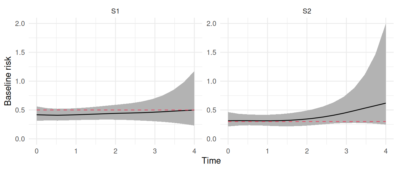
The summary shows results for the two survival outcomes, where we can see that both submodels capture the true values of treatment effect (i.e., 0.5 and -0.5, respectively). We can have a look at the baseline hazards captured in the following plot:
plot(M_cr)$Baseline +ylim(0,2)
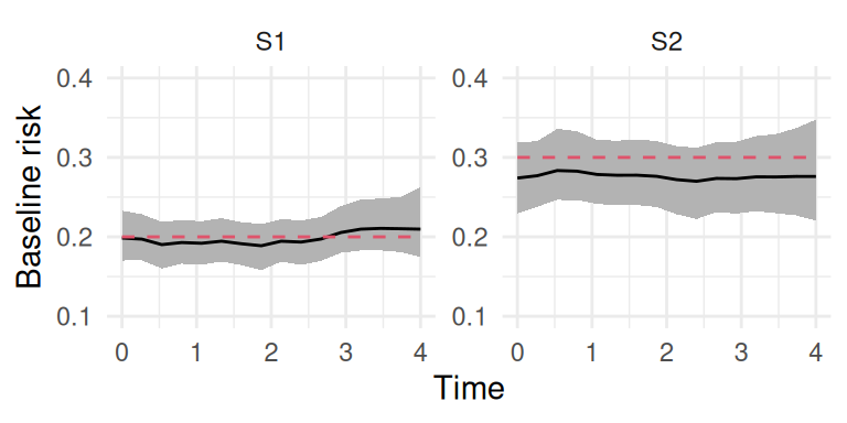
Figure 2.17: Posterior marginal distributions for the cause-specific baseline hazards for Event 1 (trt_S1) and Event 2 (trt_S2) in a competing risks model. The strainght line and shaded region indicates posterior mean and 95% credible interval while the red dashed line indicates true baseline hazard used for data generation (assumed constant for simplicity).
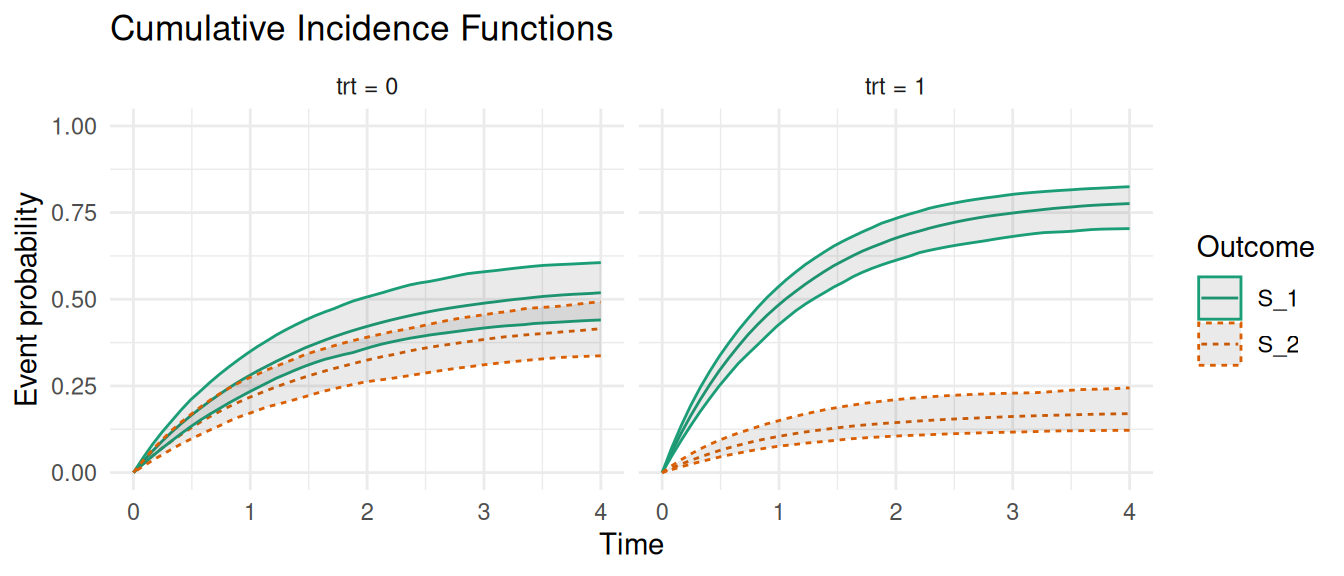
Now suppose that we want to compute the probability of experiencing a specific event over time, while accounting for the presence of other competing events. This can be obtained with the cumulative incidence function and it can be computed directly with the predict function in INLAjoint. We first create a new dataset for the scenarios of interest, here we ask for the curves for trt = 0 and trt = 1:
The new argument CIF is set to TRUE in order to compute the cumulative incidence function. CIF should be preferred over cause-specific survival functions for competing risks models as the latter corresponds to the survival probability of an event without taking into account the risk of observing the other events, which is not realistic.
Figure 2.18: Cumulative Incidence Functions (CIFs) for competing events. The plot shows the estimated CIFs for each treatment group where Event 1 is represented by the solid lines while Event 2 is represented by the dashed lines.
Here, outcome S_1 corresponds to the first event type while S_2 is the second. For example we can see that for indidividuals with trt = 0, the probability of the first event converges towards ~50% over time while for individuals with trt = 1, this probability converges towards ~75%. Note that time-dependent covariates can be included in competing risks models following the data format described in Section 2.4 and for joint models with shared time-dependent components as described in Chapter 4.
2.9 Multi-state models
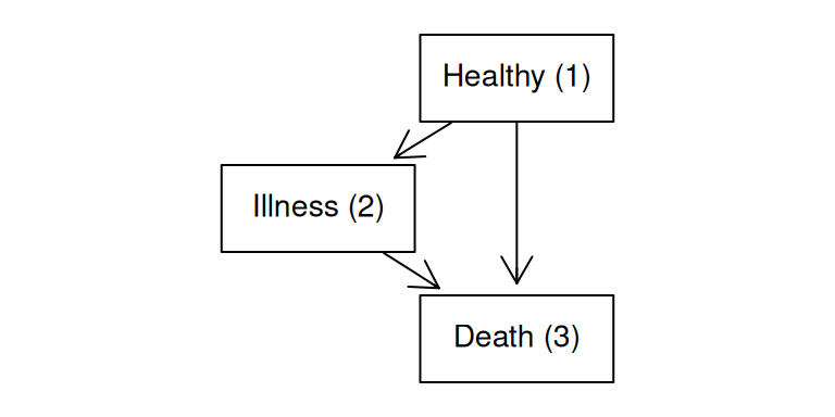
Multi-state models are used to analyze complex event histories where individuals can transition between multiple states over time. These models extend traditional survival analysis by allowing for more than two states, capturing the dynamics of transitions. In multi-state models, each state represents a distinct condition or stage, and transitions between states are governed by hazard functions that describe the instantaneous risk of moving from one state to another. These models can incorporate various types of transitions, including forward, reverse and recurrent events. Note that competing risks can be pictured as a specific case of multi-state models. Another specific and commonly used type of multi-state model is the illness-death model. This model typically consists of three states:
Healthy (or initial state): Individuals start in this state, representing the absence of disease or a baseline condition.
Illness (or intermediate state): Individuals transition to this state upon experiencing a disease or health event of interest.
Death (or absorbing state): This final state represents the end of follow-up due to death, from which no further transitions are possible.
The illness-death model allows for the estimation of transition intensities between these states, including the risk of developing the illness from the healthy state and the risk of death from either the healthy or illness state. This model is valuable for understanding the natural history of diseases and evaluating the impact of interventions. We can represent the illness-death model with a directed diagram using the graph library (Gentleman et al. (2024)):
library(graph) # just for the visual representation of multi-statenod <-c("Healthy (1)", "Illness (2)", "Death (3)")plot(graphNEL(nodes=nod, edgeL=list("Healthy (1)"=list(edges=2:3),"Illness (2)"=list(edges=3),"Death (3)"=list()),edgemode='directed'),nodeAttrs=list(shape=sapply(nod, function(x) x="box"),fontsize=sapply(nod, function(x) x=12),height=sapply(nod, function(x) x=1),width=sapply(nod, function(x) x=2)))
Figure 2.19: Illness-death multi-state model structure. This diagram illustrates the three states (Healthy, Illness, Death) and the possible transitions between them.
Each transition is represented by an arrow, and all individuals start in the Healthy (1) state. We need to define a survival model for each of these transitions. The model structure is given by the following: \[\left\{
\begin{array}{ c @{{}{}} r @{{}{}} r }
\lambda_{i,1\rightarrow 2}(t)&=\lambda_{0,1\rightarrow 2}(t)\ \textrm{exp}\left(\gamma_{1\rightarrow 2}\cdot trt_i\right) \qquad & \textbf{S1}\\
\lambda_{i,1\rightarrow 3}(t)&=\lambda_{0,1\rightarrow 3}(t)\ \textrm{exp}\left(\gamma_{1\rightarrow 3}\cdot trt_i\right) \qquad & \textbf{S2}\\
\lambda_{i,2\rightarrow 3}(t)&=\lambda_{0,2\rightarrow 3}(t)\ \textrm{exp}\left(\gamma_{2\rightarrow 3}\cdot trt_i\right) \qquad & \textbf{S3}
\end{array}
\right.\] where \(trt_i\) is a binary covariate with a different fixed effect on each transition intensity captured by the \(\gamma\) effects. Note that the baseline hazard function is transition-specific (one baseline risk for each survival model), although it is possible with INLA to use the same baseline for all transitions, this is usually done for computational ease and thus not considered relevant here.
The simulation of data from a multi-state model is similar to competing risks (since it is a special case of multi-state), although it requires to simulate data as a sequence where moving from one state to the next is based on which transition occurs first. For an illness-death model starting in the Healthy state (State 1), the simulation proceeds as follows:
For each individual, we simulate latent transition times for all possible exits from State 1. In this case, we simulate \(t_{1\rightarrow 2}\) (time from Healthy to Illness) and \(t_{1\rightarrow 3}\) (time from Healthy to Death). These are drawn from their respective transition-specific hazard models. The time of the first transition is the minimum of these latent times. If the individual transitioned to the Illness state (State 2), the simulation continues from this new state. A new latent time for the only possible exit, \(t_{2\rightarrow 3}\) (time from Illness to Death), is simulated. If the first transition was to the Death state (State 3), the process stops as it is an absorbing state. We assume that the hazard for a transition out of a state depends on the time elapsed since entering the current state (semi-markov assumption).
This first dataset contains the information for the transition from Healthy (1) to Illness (2) state. For example the second individual observe this transition at time ~3.14.
A second dataset gives the information for the transition from Healthy (1) to Death (3) state. We can see how the second individual is censored at time ~3.14 because he does observe the transition to Illness (2) state and therefore is not at risk of transition from Healthy (1) to Death (3) anymore.
The last dataset contains the information for the transition from Illness (2) to Death (3) state. This one is particular because all individuals enter in the Healthy (1) state and therefore must first transition to Illness (2) state to be at-risk of a transition from Illness (2) to Death (3) state. We therefore have an additional column here eventStart3 which gives the time of the beginning of the at-risk period. This requires to use truncation mechanism to indicate for example that individual 2 was not at risk of this transition until time ~3.14. This individual then observed the transition from Illness (2) to Death (3) state at time ~7.03.
We can now fit the illness-death model with INLAjoint, where we include a list of 3 survival formula for each transition intensity process. Since we simulated transitions between times 0 and 8 where the first transition occurs within the first 4 units of time while the transition from illness to death occurs between time 4 and 8, we need to make sure we cover the entire follow-up efficiently. The default 15 equidistant intervals may not be sufficient to capture a sequence of two event risks, therefore we manually set 100 cutpoints to have a finer resolution in the baseline hazards (in this specific example we simulated constant baseline hazards, so this will have a negligible impact but in real data application this is relevant as we don’t know the true shape of the baseline and there is no cost of having too many intervals unless for extra computation time).
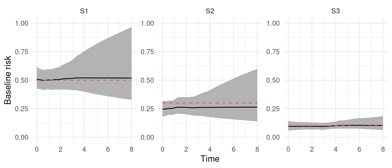
We can see that results for the effect of treatment matches with true values (i.e., 1.2, -0.2 and -1.5 for the three transitions). We can also check how the baseline hazard is captured:
plot(M_ms)$Baseline +ylim(0,1)
Figure 2.20: Posterior estimates of baseline transition hazards. The plots show the posterior mean (solid line) and 95% credible interval (shaded region) for the baseline hazards of the three transitions in the illness-death model. The estimates closely match the true constant hazards (dashed red lines) used for data simulation.
The probability of transition between states can be derived using the fitted hazard functions, which describe the instantaneous risk of moving from one state to another at any given time. We can use the predict function to compute hazard functions conditional on scenarios (e.g., trt = 0 vs. trt = 1). First we create a small dataset to describe the scenarios of interest:
ND <-data.frame("id"=1:2, "trt"=0:1);ND
  id trt
1  1   0
2  2   1
Then we call the predict function with the argument return.samples set to TRUE which keeps the samples for uncertainty quantification instead of default behavior that computes summary statistics over these samples:
P <-predict(M_ms, ND, horizon=8, id="id", return.samples=TRUE)dim(P$PredS)
[1] 300 403
Here we have 300 samples of the hazard function for each transition intensity and both scenarios, measured at multiple time points. We can derive and plot cumulative transition probabilities from these hazard functions:
Figure 2.21: Predicted transition probabilities for the illness-death model. These probabilities are derived from the multi-state model and show how the risk of moving between states evolves.
We can see how the probability of each transition evolves over time, conditional on covariate trt. Note that time-dependent covariates can be included in multi-state models following the data format described in Section 2.4 and for joint models with shared time-dependent components as described in Chapter 4. More details on multi-state models and the relationship between transition intensities and transition probabilities are available in Putter et al. (2007).
2.10 Frailty model
The frailty model is an extension of the proportional hazards model that accounts for some unobserved heterogeneity in the population. This heterogeneity, often referred to as “frailty” represents group-level variability in the risk of experiencing an event that is not explained by observed covariates. The frailty is modeled as a random effect that modifies the hazard function for each group. This random effect can follow various distributions, such as gamma or lognormal, depending on the model specification. The gamma distribution has been widely used because of the analytical solution in the likelihood of the model (it avoids having to compute the integral over the risk in the survival function). However, INLA approximate the posterior distribution for each random effect anyways and is limited to Gaussian random effects as described in Chapter 1. We therefore focus on the lognormal distribution for the frailty term in this book (i.e., a lognormal frailty corresponds to a Gaussian random effect in the linear predictor, as shown below).
When each individual have their own frailty term, it captures the unique risk profile that is not explained by included covariates (i.e., the frailty random effect captures residual noise). When individuals are grouped or clustered, such as in family studies or multi-center clinical trials. The frailty term can be shared to account for the correlation within groups, allowing for more precise inference about the effect of covariates on survival. Frailty models are particularly useful for analyzing recurrent events, where individuals can experience the same non-terminal event multiple times. In the context of recurrent events, the frailty term captures the individual-level heterogeneity in the risk of experiencing repeated events, which is not explained by observed covariates. This model is referred to as the shared frailty model, it is defined as follows: \[\lambda_{i}(t)=\lambda_{0}(t)\ \textrm{exp}\left( \gamma \cdot trt_i + v_i\right)\] where \(v_i\) represents the frailty term, with a Gaussian distribution in the linear predictor (i.e., lognormal when taken out of the exponential).
The log-normal frailty model is equivalent to a standard proportional hazards model with an additional normally-distributed random intercept added to the linear predictor. We can simulate data from this model, where the frailty term is shared among groups of individuals:
n=500# number of individualsgamma_1=1.5# treatment effectbaseScale=0.3# baseline hazard scalebaseShape=0.7# baseline hazard scalefollowup=4# study durationfrailSD <-0.5trt <-as.integer(1:n %in%sort(sample(1:n, n/2)))u <-runif(n) # uniform distribution for survival times generationw1 <-rep(rnorm(n/10, mean =0, sd = frailSD), each=10) # frailty termeventTimes <- (-(log(u))/(baseScale*exp(trt*gamma_1 + w1)))^(1/baseShape)eventTimes <-pmin(eventTimes, followup)eventIndic <-as.numeric(eventTimes<followup) # event indicatordatFr <-data.frame(id=1:n, idF=rep(1:(n/10), each=10), eventTimes, eventIndic, trt) # datasetstr(datFr)
'data.frame':   500 obs. of  5 variables:
 $ id        : int  1 2 3 4 5 6 7 8 9 10 ...
 $ idF       : int  1 1 1 1 1 1 1 1 1 1 ...
 $ eventTimes: num  0.12347 0.00451 1.78749 0.09765 4 ...
 $ eventIndic: num  1 1 1 1 0 1 1 1 1 1 ...
 $ trt       : int  1 0 0 0 0 0 0 0 0 0 ...
Here the column idF corresponds to the groups that share the same frailty term (here we assume groups of 10 individuals). The syntax to fit this model is similar to other survival models presented before but we need to add the frailty term. It can be included in the formula with the form (1|id) where 1 indicates the weight (here 1 corresponds to an intercept) and id is the grouping variable.
M_fr <-joint(formSurv =list(inla.surv(eventTimes, eventIndic) ~ trt + (1|idF)),dataSurv=datFr, id="idF")summary(M_fr)
Survival outcome
                           mean     sd 0.025quant 0.5quant 0.975quant
Baseline risk (variance) 0.1284 0.0712      0.040   0.1120     0.3139
trt                      1.5610 0.1248      1.317   1.5608     1.8063

Frailty term variance
              mean     sd 0.025quant 0.5quant 0.975quant
IDIntercept 0.3362 0.0908     0.1922   0.3247     0.5475

log marginal-likelihood (integration)    log marginal-likelihood (Gaussian)
                            -1479.262                             -1478.824

Deviance Information Criterion:  2896.159
Widely applicable Bayesian information criterion:  2898.626
Computation time: 0.62 seconds
We can see in the results the effect of treatment that matches with the true value (1.5) while the frailty term is described by its variance. This variance quantifies the degree of unobserved heterogeneity within the population. It tells us how much the underlying risk varies between groups (or individuals) after accounting for all the measured covariates in the model. It is however easier to interpret standard deviations rather than variances. We can convert the variance of the frailty random effect to a standard deviation (\(\sigma\)) by adding the argument sdcor=TRUE to the call of the summary function:
summary(M_fr, sdcor=TRUE)
Survival outcome
                           mean     sd 0.025quant 0.5quant 0.975quant
Baseline risk (variance) 0.3463 0.0921     0.1999   0.3347     0.5603
trt                      1.5610 0.1248     1.3170   1.5608     1.8063

Frailty term standard deviation
              mean     sd 0.025quant 0.5quant 0.975quant
IDIntercept 0.5747 0.0768     0.4384   0.5698     0.7399

log marginal-likelihood (integration)    log marginal-likelihood (Gaussian)
                            -1479.262                             -1478.824

Deviance Information Criterion:  2896.159
Widely applicable Bayesian information criterion:  2898.626
Computation time: 0.62 seconds
Since the frailty term is assumed to be normally distributed on the log-hazard scale, approximately 95% of the groups will have a frailty term between \(−1.96*\sigma\) and \(+1.96*\sigma\). This can be translated into a range of hazard ratios relative to the median group (which has a frailty of 0 and a hazard ratio of exp(0)=1).
For example, a group at the 2.5th percentile of frailty has a hazard that is exp(-1.96*0.57) = 0.327 times the hazard of the median group. On the other hand, a group at the 97.5th percentile of frailty has a hazard that is exp(1.96*0.57) = 3.055 times the hazard of the median group. Therefore, we can conclude that there is substantial unobserved heterogeneity, with the risk of the event varying by a factor of roughly 9 between the least and most frail groups in the population, due to factors not captured by the measured covariates.
We can plot the posterior marginal distributions for the standard deviation of the frailty as well as the baseline hazard:
Here we can see how the first group has a higher risk of event compared to population average while the second group has a lower risk. Finally, we can use the predict function to compare the survival probabilities conditional on covariates while accounting for the frailty. Let’s consider two scenarios for each trt line:
Here we assume the new individuals we predict for are associated to an independent draw from the posterior marginal distribution of \(v_i\) (i.e., idF=1,2 is treated as two individuals that each belong to a new frailty group). It is also possible to predict conditional on the new individual belonging to an already existing group of the frailty random effect (e.g., a frailty term is assumed for different cities and the new individual belongs to one of the city we learned from). Let’s consider our two individuals belong to frailty group 1 vs. group 2. We need to first draw samples from the conditional posterior of the corresponding frailty group, which is done with inla.posterior.sample, where we can select draws from the posterior distribution of the frailty group of interest (here the first two ids of the frailty random effect named ID_Intercept_S1). Then, we call the predict function where the pre-sampled conditional frailty values are directly provided in the set.samples argument of the predict function. Internally, INLAjoint uses these samples instead of assuming a new draw from the posterior distribution of the random effect:
Figure 2.23: Survival probability predictions from the frailty model comparing marginal predictions (left) with group-specific predictions for frailty groups 1 (center) and 2 (right).
We can see that using the information from a frailty group from which we already learned makes predictions more accurate compared to when we assumed the individuals belongs to a new frailty group from which we don’t know anything.
2.11 Joint frailty model
The frailty term that is captured in a shared frailty model corresponds to a deviation from the average risk. This frailty term could be shared in another submodel in order to capture the effect of being higher at risk for an event on the risk of another event. This is referred to as the joint frailty model (Rondeau et al. (2007)). While in the previous section the frailty was shared within groups of individuals with an unique event time, here we show how the frailty term can also be used to model recurrent events.
For example if we consider the risk of going to the hospital for individuals that may visit the hospital multiple times, a frailty term can capture how frail is each individual, where individuals with multiple visits to the hospital are associated to a higher frailty compared to individuals that never visit the hospital. This captured frailty could be shared in a second survival model that evaluates the effect of covariates on the risk of death, where the frailty term can be shared in order to evaluate if an individual with a higher risk of going to the hospital is associated to a higher risk of death for example. Let’s consider the following model \[\left\{\begin{array}{ c @{{}{}} r @{{}{}} r }\lambda_{i1}(t)=\lambda_{01}(t)\ \textrm{exp}\left(\gamma_{11}\cdot trt_i + v_i \right) \qquad & \textbf{S1}\\
\lambda_{i2}(t)=\lambda_{02}(t)\ \textrm{exp}\left(\gamma_{21}\cdot trt_i + \gamma_{22}\cdot v_i \right) \qquad & \textbf{S2}\\
\end{array}\right.\] where the first model corresponds to the risk of recurrent events for individual \(i\) while the second model corresponds to the risk of another event of interest for individual \(i\). The covariate trt is a binary covariate that affect the risk of both events through risk-specific fixed effects \(\gamma_{11}\) and \(\gamma_{21}\). The frailty term \(v_i\) captures the individual deviation from the average risk of the recurrent event and also affects the risk of the second event, scaled by the fixed effect \(\gamma_{22}\).
We can simulate data from this model, first we simulate recurrent events:
For simplicity we limit the number of recurrent events for each individual to 3 and we assume calendar times (time to event), although switching to gap times (i.e., time between events) is straightforward.
Now, we can simulate another event time that depends on the frailty scaled by a fixed effect:
gamma21=-0.5# trt effect second eventgamma22=1# frailty effect second eventbaseScale2=0.3# baseline hazard scale second eventeventTimes2 <--(log(runif(n))/(baseScale2*exp(trt*gamma21 + w1*gamma22)))eventIndic2 <-as.numeric(eventTimes2<followup)eventTimes2 <-pmin(eventTimes2, followup)datFrJ2 <-data.frame("id"=1:n, "trt"= trt,"eventTimes2"= eventTimes2,"eventIndic2"= eventIndic2)head(datFrJ2)
We have two datasets because datFrJ contains multiple lines per individuals (recurrent events) while datFrJ2 contains an unique event time per individual. Of note, here the second event is assumed not terminal.
The formSurv argument for this model is similar to the competing risks and multi-state models as it involves a list of formulas for each event outcome. Here we have the first formula for recurrent events that includes the frailty term, where inla.surv includes the argument subject for the data expansion to account for individual recurrent events. The second formula corresponds to the second event where the frailty term is shared and scaled.
The parameter assocSurv indicates that the frailty term from the recurrent event model is shared in the second event model, if it was set to FALSE, then the frailty term would only be included in the first submodel. The order is important, the first model in the list of survival formulas (formSurv) should include a random effect and it can be shared in the next formulas. Multiple survival models with random effects can be accommodated and a random effect can be shared in multiple survival models (i.e., this argument should be a vector of booleans if one random effect is shared in multiple survival submodels and a list of vectors if multiple survival models with random effects share their random effects in multiple survival models).
We can see that the model is able to capture the true values of the parameters, such as the fixed effect of treatment on first (1.2) and second (-0.5) outcomes. The association parameter links the two survival processes, when positive, individuals or groups with a higher hazard rate for the recurrent event (i.e., a higher frailty term) also have a higher hazard for the second event. A negative value means that a higher risk for the recurrent event is associated with a lower risk for the second event. If the credible interval contains zero, there is no statistical evidence of an association between the two processes, conditional on the covariates.
The estimated posterior mean for the association is 0.975, which is a log-hazard ratio. We can directly get the hazard ratio by adding the argument hr=TRUE to the call of the summary function:
A one-unit increase in the log-frailty for the recurrent event is associated with a hazard ratio of 2.726 for the second event.
After accounting for the effect of treatment, there is strong evidence for a positive association between the two event processes. Specifically, a one-unit increase in the subject-specific log-frailty for the recurrent event is associated with a 173% increase on average (95% CI: [70%, 327%]) in the hazard for the second event. This suggests that common unobserved factors drive the risk for both types of events.
We can also display the baseline hazard for each outcome as well as the posterior marginal of the standard deviation of the frailty:
Figure 2.25: Survival probability predictions from the joint frailty model for both recurrent events (S1) and terminal events (S2), showing different treatment effects on each type of event.
We can also compute the probability of observing the second event type conditional on recurrent observations of the first event. In order to do so, let’s assume one individual observe 3 recurrent events during the follow-up at time 0.3, 0.6 and 1 while another individual is censored without observing any recurrent events at time 1, we predict at horizon 4:
Figure 2.26: Conditional survival probability predictions from the joint frailty model comparing individuals with different recurrent event histories. The individual with 3 recorded recurrent events (left) shows lower survival probabilities than the individual with no recorded events (right), reflecting the positive association between event types.
We can see how the individual that observed some recurrent events is associated to a higher frailty compared to the other individual, leading to lower survival probabilities for both events (as a higher risk of the first event is associated to a higher risk of the second event since the association \(\gamma_{22}\) is positive). These two plots presented in Figure 2.26 show respectively higher/lower survival probabilities compared to the population average shown in Figure 2.25 since they represent scenarios associated to opposite deviations from the population average.
2.12 Prior distributions for survival models
Prior distributions represent the initial beliefs or knowledge about the parameters of the model before observing the data. As discussed in Chapter 1, they are updated once data is observed according to Bayes theorem to get posterior distributions. Informative priors reflect strong beliefs or existing knowledge about the parameters range of plausible values, based on previous studies or expert opinion. Weakly informative priors, on the other hand, are vague and allow the data to dominate the inference process. However, excessively vague priors can have detrimental effects, so it is preferable to use a prior that puts more mass on a plausible range of values. In this section we present the default priors used for the models described in the rest of this chapter, and we show how to modify these default priors.
The default priors in INLAjoint are weakly informative, although for some parameters the notion of prior informativeness can be tricky. Depending on the scale of the observed data, and the desired behavior of the prior that may be based on the research question of interest, the default priors of INLAjoint could be too informative or not informative enough.
2.12.1 Fixed effects
Fixed effects are assigned a Gaussian prior with mean 0 and variance 100 (which is a vague prior for scaled covariates). It is possible to display the priors of a fitted model with the function inla.priors.used for any R-INLA or INLAjoint object, or directly by looking at the argument priors_used for INLAjoint objects. For example we can check the priors for the fixed effects of the first model fitted with INLAjoint in Section 2.2.1:
There are 2 elements corresponding to the mean and precision (i.e., inverse of variance) for the fixed effects. These can be changed in the control options of INLAjoint when fitting the model:
Here, although we set a more informative prior (\(\mathcal{N}(\mu=-1, \sigma^2=1)\)) on the fixed effects compared to default \(\mathcal{N}(\mu=0, \sigma^2=100)\), it still includes the true values (log(0.2) for the exponential rate and 0.2 for the treatment effect) in the plausible area and thus when updating priors with the observed data, we recover the true value of the exponential rate and treatment effect in the posterior. The posterior here is mostly data-driven.
Figure 2.27: Comparison of prior (black solid) and posterior (red dashed) distributions for the exponential baseline rate (left) and treatment effect (right). The blue dotted lines show the true values. The posteriors are largely data-driven.
INLAjoint’s plot function allows to display the priors and posterior distribution of covariates effects by adding the argument priors=TRUE to the call of the plot function:
plot(M_exp2, priors=TRUE)$Outcomes[[1]]
Figure 2.28: Prior and posterior distributions displayed using the INLAjoint plot function with priors=TRUE. This provides a convenient way to visualize the impact of prior specification on parameter estimation.
We can set an informative prior \(\mathcal{N}(\mu=-10, \sigma^2=0.01)\) which is incompatible with the true value that generated the data:
Figure 2.29: Impact of a misspecified informative prior. This figure illustrates the effect of using a strong but incorrect prior for the treatment effect and the exponential baseline rate. The posterior distributions (dashed lines) are heavily influenced by the misspecified priors (solid lines) and fail to capture the true parameter values (vertical dotted lines), illustrating the risks of overly confident prior specifications.
We can see that with such an informative prior, the posterior is not matching the true value anymore. There is not enough data to overcome the amount of information given by the prior.
It is also possible to set a different prior for each fixed effect, in order to do so we need to use the “build only” technique introduced in Section 1.5.8. We first create the model in INLAjoint, and then assign different priors for each fixed effect, whereafter we can run the model in R-INLA, as illustrated next.
Figure 2.30: Posterior distributions with user-defined priors in INLAjoint. The plot shows the posterior distributions (dashed lines) for the treatment effect and the exponential baseline rate where the priors are displayed as solid lines. The posteriors are centered around the true parameter values (vertical dotted lines).
2.12.2 Baseline hazard parameters
We showed how the log-rate of the exponential baseline is considered as a fixed effect (i.e., the value of the linear predictor when all covariates are zero). In Section 2.2.2, we have introduced the parametric Weibull baseline hazard which involves two parameters, where the scale is defined as the rate of the exponential and the shape of the Weibull is considered as an hyperparameter. The prior for this hyperparameter can be tricky as it is not easy to figure out what a non-informative distribution would mean for such a parameter. INLA defines a PC prior for this parameter, see Van Niekerk et al. (2021) for a detailed discussion of the choice of INLA’s prior for this shape parameter.
The base model for the Weibull distribution is the simpler exponential distribution, which corresponds to a shape parameter \(\alpha=1\). This represents a constant hazard over time. The PC prior penalizes the model’s complexity as it deviates from this exponential base model. In practice, this means the prior will shrink the shape parameter toward 1, favoring a constant hazard unless there is evidence in the data for an increasing (\(\alpha > 1\)) or decreasing (\(\alpha < 1\)) hazard. This principled shrinkage helps to prevent overfitting and ensures that the more flexible Weibull model can revert to the simpler exponential model when the data supports it, a property that is not guaranteed with other common prior choices like the Gamma distribution. See inla.doc("pc.alphaw") for more details on this prior and default options with INLA.
For the random walk baseline, the model involves an additional parameter for the precision of the random walk which is assigned a PC prior, i.e., \(P(\sigma>\sigma_0) = p\), where \(\sigma_0\) and \(p\) are user-defined. This is an intuitive prior that interprets as “the probability of the parameter having a higher value than \(\sigma_0\) is \(p\)”. Default values are \(\sigma_0=0.5\) and \(p=0.01\). For example we can have a look at the prior used in the random walk of order 2 model fitted in Section 2.2.3:
M_rw2$priors_used$priorRW
[1] 0.50 0.01
And we can modify this prior, although the default option is usually a good choice for these parameters where there is no intuition on the desired behavior of the prior.
More generally, priors can be freely modified to any available distribution in INLA (including the possibility for the user to implement new priors, see Chapter 5 of Gómez-Rubio (2020)).
2.12.3 Frailty random effect
The variance of the frailty random effects are assigned by default an inverse-Gamma prior \(IG(\alpha=4, \beta=1)\). We can check the priors from the model fitted in Section 2.10:
M_fr$priors_used$priorFrailty
$alpha
[1] 4

$beta
[1] 1
The parameters \(\alpha\) and \(\beta\) of this prior can be changed in control options:
It is also possible to display the prior and posterior distributions of the variance with the boolean argument priors in the call of the plot function:
plot(M_fr2, priors=TRUE)$Covariances$L1
Figure 2.31: Prior (dashed line) and posterior (solid line) for the variance parameter of a frailty term in a proportional hazards model.
It can also be displayed as standard deviation using the argument sdcor=TRUE:
Figure 2.32: Prior (dashed line) and posterior (solid line) for the standard deviation of a frailty term in a proportional hazards model.
Finally, it is possible to switch to a PC prior for the variance of the frailty, although not directly available in INLAjoint it can be switched using the “build only” trick introduced in Section 1.5.8. The code below demonstrates this process by first setting up the model without running it (run=FALSE), and then manually modifying the underlying INLA formula. The key change is to replace the default random effect with an f() term that explicitly specifies the PC prior for the precision (prior = "pc.prec"). This prior is defined by the user-defined parameters param = c(1, 0.01), which sets the prior based on an intuitive statement about the standard deviation of the frailty (i.e., the probability that the variance of the frailty random effect is higher than 1 is 1%):
M_fr30 <-joint(formSurv =list(inla.surv(eventTimes, eventIndic) ~ trt + (1|idF)),dataSurv=datFr, id="idF", run=F)M_fr30$.args$formula <-as.formula(paste(c("Yjoint ~ -1 ",attr(terms(M_fr30$.args$formula), which ="term.labels")[1:3],"+ f(IDIntercept_S1, WIntercept_S1, model = \"iid\", n = 50, hyper = list(prec = list(prior = \"pc.prec\", param = c(1, 0.01))))"), collapse="+"))M_fr3 <-joint.run(M_fr30)summary(M_fr3)
Survival outcome
                           mean     sd 0.025quant 0.5quant 0.975quant
Baseline risk (variance) 0.1282 0.0711     0.0398   0.1118     0.3137
trt                      1.5609 0.1256     1.3153   1.5607     1.8077

Frailty term variance
              mean     sd 0.025quant 0.5quant 0.975quant
IDIntercept 0.3385 0.1005     0.1814   0.3253      0.574

log marginal-likelihood (integration)    log marginal-likelihood (Gaussian)
                            -1481.139                             -1480.708

Deviance Information Criterion:  2896.449
Widely applicable Bayesian information criterion:  2898.933
Computation time: 0.67 seconds
The pc priors here may be useful to overcome some issues related to the inverse-Gamma distribution for variance parameters, see Sterrantino et al. (2025).
Alvares, D., Van Niekerk, J., Krainski, E. T., Rue, H., & Rustand, D. (2024). Bayesian survival analysis with INLA. Statistics in Medicine, 43(20), 3975–4010. https://doi.org/10.1002/sim.10160
Anderson-Bergman, C. (2017). icenReg: Regression models for interval censored data in R. Journal of Statistical Software, 81(12), 1–23. https://doi.org/10.18637/jss.v081.i12
Fisher, L. D., & Lin, D. Y. (1999). Time-dependent covariates in the cox proportional-hazards regression model. Annual Review of Public Health, 20(1), 145–157. https://doi.org/10.1146/annurev.publhealth.20.1.145
Garcı́a-Hernandez, A., Pérez, T., Pardo, M. del C., & Rizopoulos, D. (2020). MMRM vs joint modeling of longitudinal responses and time to study drug discontinuation in clinical trials using a “de jure” estimand. Pharmaceutical Statistics. https://doi.org/10.1002/pst.2045
Gentleman, R., Whalen, E., Huber, W., Falcon, S., Gentry, J., & Shannon, P. (2024). Graph: A package to handle graph data structures. https://doi.org/10.18129/B9.bioc.graph
Gressani, O., Faes, C., & Hens, N. (2022). Laplacian-p-splines for bayesian inference in the mixture cure model. Statistics in Medicine, 41(14), 2602–2626. https://doi.org/10.1002/sim.9373
Holford, T. R. (1976). Life tables with concomitant information. Biometrics, 32(3), 587–597. https://doi.org/10.2307/2529747
Ibrahim, J. G., Chu, H., & Chen, L. M. (2010). Basic concepts and methods for joint models of longitudinal and survival data. Journal of Clinical Oncology: Official Journal of the American Society of Clinical Oncology, 28(16), 2796–2801. https://doi.org/10.1200/JCO.2009.25.0654
Johansen, S. (1983). An extension of cox’s regression model. International Statistical Review / Revue Internationale de Statistique, 51(2), 165–174. https://doi.org/10.2307/1402746
Neto, D. S., Rustand, D., Rue, H., Alvares, D., & Tomazella, V. L. (2025). A new approach for bayesian joint modeling of longitudinal and cure-survival outcomes using the defective gompertz distribution. arXiv Preprint arXiv:2507.23196. https://doi.org/10.48550/arXiv.2507.23196
Putter, H., Fiocco, M., & Geskus, R. B. (2007). Tutorial in biostatistics: Competing risks and multi-state models. Statistics in Medicine, 26(11), 2389–2430. https://doi.org/10.1002/sim.2712
Rondeau, V., Mathoulin-Pelissier, S., Jacqmin-Gadda, H., Brouste, V., & Soubeyran, P. (2007). Joint frailty models for recurring events and death using maximum penalized likelihood estimation: Application on cancer events. Biostatistics, 8(4), 708–721. https://doi.org/10.1093/biostatistics/kxl043
Royston, P., & Parmar, M. K. (2002). Flexible parametric proportional-hazards and proportional-odds models for censored survival data, with application to prognostic modelling and estimation of treatment effects. Statistics in Medicine, 21(15), 2175–2197. https://doi.org/10.1002/sim.1203
Rustand, D., Van Niekerk, J., Rue, H., Tournigand, C., Rondeau, V., & Briollais, L. (2023). Bayesian estimation of two-part joint models for a longitudinal semicontinuous biomarker and a terminal event with INLA: Interests for cancer clinical trial evaluation. Biometrical Journal, 65(4), 2100322. https://doi.org/10.1002/bimj.202100322
Spiegelhalter, D. J., Best, N. G., Carlin, B. P., & Van Der Linde, A. (2002). Bayesian measures of model complexity and fit. Journal of the Royal Statistical Society B: Statistical Methodology, 64(4), 583–639. https://doi.org/10.1111/1467-9868.00353
Sterrantino, A. F., Rustand, D., Niekerk, J. V., Krainski, E. T., & Rue, H. (2025). A graphical framework for interpretable correlation matrix models. arXiv Preprint arXiv:2312.06289. https://doi.org/10.48550/arXiv.2312.06289
Tsiatis, A. A., Degruttola, V., & Wulfsohn, M. S. (1995). Modeling the relationship of survival to longitudinal data measured with error. Applications to survival and CD4 counts in patients with AIDS. Journal of the American Statistical Association, 90(429), 27–37. https://doi.org/10.2307/2291126
Van Niekerk, J., Bakka, H., & Rue, H. (2021). A principled distance-based prior for the shape of the weibull model. Statistics & Probability Letters, 174, 109098. https://doi.org/10.1016/j.spl.2021.109098
Van Niekerk, J., Bakka, H., & Rue, H. (2023). Stable non-linear generalized bayesian joint models for survival-longitudinal data. Sankhya A.
Van Niekerk, J., & Rue, H. (2022). Use of the INLA approach for the analysis of interval-censored data. In Emerging topics in modeling interval-censored survival data (pp. 123–140). Springer.
Wang, Y., & Taylor, J. M. G. (2001). Jointly modeling longitudinal and event time data with application to acquired immunodeficiency syndrome. Journal of the American Statistical Association, 96(455), 895–905. https://doi.org/10.1198/016214501753208591
Whitehead, J. (1980). Fitting cox’s regression model to survival data using GLIM. Journal of the Royal Statistical Society C (Applied Statistics), 29(3), 268–275. https://doi.org/10.2307/2346901
Xu, C., Hadjipantelis, P. Z., & Wang, J.-L. (2020). Semi-parametric joint modeling of survival and longitudinal data: The r package JSM. Journal of Statistical Software, 93(2). https://doi.org/10.18637/jss.v093.i02